Amount of RAM in the system	Recommended swap space	Recommended swap space if allowing for hibernation
⩽ 2 GB	2 times the amount of RAM	3 times the amount of RAM
> 2 GB – 8 GB	Equal to the amount of RAM	2 times the amount of RAM
> 8 GB – 64 GB	At least 4 GB	1.5 times the amount of RAM
> 64 GB	At least 4 GB	Hibernation not recommended

Modern RAM is dynamic RAM or DRAM. This is made of one transistor + capacitor per bit. DRAM is cheap and dense, but loses the value after a few milliseconds unless refreshed (read and re-written) before then. Fast DRAM can have errors. Adding parity bits (ECC or error correcting code) is used in servers used in data centers, when the cost is worth not having errors.

Studies done in 2015 have shown DRAM errors are often caused by one bad cell in a row or column of a memory block. Facebook and others have added page retirement, which is the same as mapping out bad blocks on a disk, but for RAM.

Static RAM or SRAM uses 6 transistors per bit and is nearly twice as expensive as DRAM, but doesn’t need to be refreshed and so uses less power and is around 6 times faster.

RAM is sold in modules called DIMMs (dual inline memory modules) that plug into mating sockets on the motherboard. This allows RAM to be upgraded or replaced as needed. The speed of RAM is measured in terms of the original speed: DDR (double data rate), DDR2 (double DDR) and DDR3 (double DDR2). In 2012, the DDR4 standard was finalized; it operates at a maximum of 1.2 volts (20 percent less voltage than DDR3), and achieves data transfer rates of 3.2 billion transfers per second (double DDR3). As of 2018, DDR5 is available and DDR6 has been announced.

RAM sold for use on servers often includes extra parity bits per byte, so the RAM can detect any errors and, in some cases, correct them. This “EC” RAM is a lot more expensive than commodity DRAM used in PCs.

RAM can have some performance issues an SA should know about.

· Most RAM is for dual channel use, which requires DIMMs to be installed in identical pairs and in specific slots on the motherboard. This doesn’t always happen at the factory, and then the BIOS will default to single channel mode, halving the speed! You should visually inspect that the RAM is installed correctly.

· Another issue is that RAM reports to BIOS on POST its maximum speed (using SPD or XMS method), but some BIOSes will ignore that and default to some safe, slow speed! You can sometimes set BIOS parameters to override that, to get the maximum speed you paid for.

· Finally, the speed of the RAM and CPU is used by the BIOS to set the bus speed. Cheaper RAM has fewer operating speeds (“modes”), and this limits the CPU multiplier that can be used, thus slowing the whole bus. Suppose you have a 2.4 GHz CPU. Using 667 MHz DDR2 RAM will end up setting the bus to 300 MHz (and a CPU multiplier of 8). Upgrading to 800 MHz DDR2 will result in a bus speed of 400 MHz (and a 6x CPU multiplier).

This table from an Ars Technica post shows the memory hierarchy:

Level Access time Typical size

Registers "instantaneous" under 1KB

Level 1 Cache 1-3 ns 64KB per core

Level 2 Cache 3-10 ns 256KB per core

Level 3 Cache 10-20 ns 2-20 MB per chip

Main Memory 30-60 ns 4-32 GB per system

Hard Disk 3,000,000-10,000,000 ns over 1TB

Devices Often called peripherals, these include keyboard, video controllers, ports, IDE/SCSI controllers, sound, clock, ...). Peripherals generally require a controller; the device connects to the controller, which is installed in the computer (using some add-on slot) and connected to the system bus.

Keyboard Input Keyboards don’t (any longer) send ASCII when any (combination of) keys are struck. For one thing, many keys have no ASCII (or even Unicode) equivalent (e.g., pgUp). Instead, the keyboard sends numbers known as scancodes. These are only roughly standardized. If you have an unusual keyboard you can use the setkeycodes(8) command to remap some scancodes in the tty driver. (The first 88 scancodes cannot be re-mapped.)

The kernel’s tty driver also contains a table called the keymap (see keymaps(5)) that translates scancodes to standard key names called keycodes. Software sees keycodes on key-pressed/released events. You can see scancodes and keycodes in a non-GUI console window using showkey(1) command.

Many standard keymaps are available for different keyboards (e.g., UK keyboards, German keyboards, etc.) The keymap translates sequences of scancodes into keycodes. Use loadkeys(1) / dumpkeys(1) to change/view the keymap table. (e.g., disable/move caps lock, define function and other extra keys, etc.

The keyboard driver translates keycode sequences into Unicode (e.g., ALT+,+c = ç) or some action (e.g., CTL+C sends a signal), determines what strings to send when function keys are pressed, and the effects of modifier (shift, alt, etc.) keys.

The readline(1) library, used by shell, mysql, psql, ..., allows you to bind keycodes to arbitrary meanings (e.g., symbols, Unicode, shell commands, etc.) with bind or ~/.inputrc. It is readline that provides a history mechanism for these commands, and allows input editing.

Finally keep in mind this console tty driver isn’t used for USB keyboards, remote SSH sessions, or GUI (X window) sessions, so updating scancodes or keymaps has no effect in these cases. (X has its own keyboard driver and you can remap its keycode table using xmodmap, discussed later.)

Solaris/Sparc systems use keyboards with an extra key, “STOP”. During the boot process you take control by hitting keys such as “STOP-A” (the STOP and the A key simultaneously).

Networking Hardware

Stuff you should know: NICs, static (manually set) versus dynamic (automatically set) networking information (parameters) including IP address, mask, default gateway IP address (default route), DNS server(s) (up to 3) IP addresses, DNS hostname, DNS domain-name, (FQDN), and default DNS domain name. Usually set dynamically with DHCP. (Discuss many “hostnames” issue: NIS, per system, NetBIOS, or DNS. Similar issues with “domain-name”.) RH GUI tools get these confused and won’t always work.

How can you tell which hardware will work with your OS? Proprietary Unix (not to mention Mac and Windows) vendors maintain hardware compatibility lists. Some major Linux vendors do as well (such as Red Hat). However, many users send hardware compatibility reports to various places that anyone can check, such as smolts.org or the ones listed at linux-drivers.org.

System Clock

Traditionally, hardware generates a tick event every so often; this is the CPU (and FSB if you have one) clock speed, often 3GHz or more today.

The kernel maintains a software clock known as the system clock with a lower resolution: every so many hardware ticks, a software tick count is incremented. This counter is the system clock used by the date command.

The tick frequency can be adjusted in some cases to better match graphic card processing speeds (for serious gamers). In Linux, this is controlled by the kernel value HZ, which in turn sets the duration of a software clock tick called a jiffy. (See time(7).) On Linux, a jiffy is usually 4 mSec. (On Windows 7, it is 15.6 mSec.) (In short: the hardware generates ticks, counted by the kernel, and every so many hardware ticks (depending on HZ) a software tick event is generated and the system clock updated.)

A problem with this scheme is that the CPU must handle a tick event every jiffy. Processors these days all have power management capabilities. When they have no work to do, they can be put into some low-power state, drastically reducing their power consumption. The more time they can spend asleep, the less power they use. With this kind of processor, that periodic tick is a liability. It means that even when the processor has nothing useful to do, it will be awakened every jiffy just to update a counter and then go back to sleep.

For some time now, most kernels support tickless kernels, also known as dynamic tick. Linux integrated support for this in 2007, and more recently OS X is also tickless. Windows 8 is tickless too. With a tickless kernel, instead of indiscriminately making the timer fire every few milliseconds the kernel takes a look at all the timed events outstanding. It then sets the timer for the earliest timed event it has to wait for. So if the shortest wait the system has to attend to is 200 milliseconds, then the timer will be set for 200 milliseconds. This allows the CPU to remain in the low power state longer.

Power-On Cycle

When the power is turned on, the CPU starts executing a firmware program (often called BIOS) stored in nonvolatile memory. (Newer systems have replaced BIOS with EFI, discussed later.) (FYI: BIOS starts at address 0xFFFF0, not 0 as you might have expected.) BIOS varies by motherboard brand. Often the term system firmware (or just firmware alone) is used to refer to this BIOS/EFI firmware.

The first thing the firmware does is to detect and test the hardware. After this POST (power on self-test), the BIOS finds and initializes keyboard and monitor. (Sometimes, part of the POST runs after the monitor is initialized, so results can be displayed.) The CMOS memory (a type of volatile RAM backed by a battery) holds various settings) is examined and the settings stored there are applied. Boot devices (and some other hardware such as the bus controller, the keyboard controller, etc.) are located and initialized.

Finally, the operating system kernel must be found and loaded into RAM. With traditional BIOS and DOS disks, the MBR of the first disk on the first controller is examined for a kernel loader program; if not found then the loader in the active partition’s boot blocks is used. If none is found there either, the disk is not bootable and other disk drives may be tried.

In the past, BIOS has been proprietary firmware provided by the motherboard manufacturer. OpenBoot is BIOS defined by IEEE Standard 1275-1994, Standard for Boot Firmware, and is used on Solaris SPARC and a few other server platforms. (See Solaris console operations or the Solaris OpenBoot Reference Manuals for more info.) For Linux, a group of developers wanted a non-proprietary version and started the LinuxBIOS project, now called coreboot. However, all of this BIOS stuff has been displaced by newer firmware called UEFI (discussed later).

This firmware is executed immediately after you turn on your system. See man pages for kernel, eeprom. The OpenBoot firmware can be configured for interactive booting; it will pause for user instructions after the POST; the prompt is “ok> ”.

Related to the power supply are the features suspend and hibernate.

Suspend means to put the DRAM (main memory) into a low-power state, and shut down as much of the rest of the computer as possible. You can leave a laptop or desktop in suspend, but it will slowly drain the batteries of a laptop unless plugged into a recharger.

Hibernate saves the content of your RAM to the hard drive using swap space, then shuts down the computer completely. This feature is unavailable unless you configure enough swap space.

Laptops can benefit from a hybrid approach that saves memory to disk, then suspends. If the battery runs out, your PC can resume from hibernate; otherwise it resumes from suspend.

The primary tasks of the system firmware are to:

· Determine the hardware configuration

· Test (POST) and initialize the system hardware (Qu: What hardware?)

· Provide interactive debugging facilities for testing hardware and software, for setting the hardware clock, and for changing CMOS settings

· Boot the operating system from either a mass storage device or from a network, using an OS loader (that the firmware searches for)

OS loader (or boot loader or boot manager) is located by the system firmware in order to load the actual operating system into memory. For older BIOS/DOS disks, the loader is read from the MBR (Master Boot Record) of the selected boot device, if present. If not, the firmware looks in the boot block of the active partition for a loader (used with dual booting).

For EFI/GPT disks, the boot loader is just a program that can be read from the disk, often called grub.efi or elilo.efi. (Not having to fit the loader into a single disk sector is one advantage of EFI.)

A feature of UEFI is secure boot, which requires the hardware check the digital signature of firmware, then have the firmware check the digital signature of the kernel. Microsoft made a deal with some hardware vendors to include only its public key in hardware.

To support Linux, Ubuntu and Red Hat have developed a “shim” boot loader, signed by Microsoft, which in turn loads GRUB (the regular boot loader). The Linux foundation has developed a pre-loader loader that is similar to the shim loader, only it doesn’t check the signature of the full loader (GRUB).

On some systems you can change a CMOS setting to disable secure boot.

Some common OS loaders for Linux that work with other systems as well (MS, Solaris) are LILO (and the EFI version, elilo) and GRUB (the most common today). loadlin.exe is used when HW must be initialized from DOS drivers (very rare anymore). PowerPC systems use yaboot. Also common is efilinux.

An excellent source of information on boot loaders (and in particular, for UEFI) can be found at rodsbooks.com.

For bootable removable media, such as bootable CDs, DVDs, Flash, etc., the ISOLINUX boot loader is often used. (It is related to other loaders from the same group, SYSLINUX).

To see which loader is in use for MBR disks, run bootinfoscrypt:
sudo bootinfoscript --stdout | awk '/______________/ {exit}; {print $0}'

GRUB is used directly by PCs using traditional BIOS boot. However, some PCs do not support BIOS boot anymore, only UEFI boot.

The open source firmware Das U-Boot contains a partial implementation of the UEFI specification. (A complete open source implementation is offered by TianoCore EDK II. Companies like Phoenix offer closed source UEFI firmware.)

On the 64-bit ARM architecture, Some Linux distributions such as SuSE and Fedora use U-Boot to load GRUB as a UEFI application from U-Boot. GRUB in turn loads and starts the Linux kernel via UEFI API calls. Note Linux itself has an UEFI stub so it can be started as a UEFI application on Intel x64 architectures.

Because the MBR or boot block is limited in size (446 bytes for the loader code), BIOS-based OS loaders have two (or more) stages. Only the first stage is in the boot block/MBR. This software locates and loads the second stage loader from someplace, often the unused space between the MBR and the first partition, or in the boot partition, which can be a much larger program. (The initial stage is so small, it used BIOS calls to read sectors using LBA addresses.) This first stage loads a second stage, which may load another stage, which in turn actually loads the OS, according to its configuration. With GRUB, the second stage is considered part of the first one; both together are called the Grub core. That loads Grub modules, usually filesystem drivers. Mention coreboot (formerly LinuxBIOS), with a 3 second boot (!), mkbootdisk, uname (and who -r).

Even before an OS is loaded, some firmware may be available to control the boot process, perform remote management functions, and various configuration tasks. This firmware is usually called LOM, or Lights Out Management.

LOM is the standard system controller for remote out-of-band management (often uses a separate, dedicated NIC) for many types of servers and some Apple computers and PCs. The hardware involved is usually called the baseboard management controller or BMC. The BMC is usually a system on a chip (SoC) that you find in various devices and smartphones.

LOM functions include monitoring, logging, alerting, and basic control of the system. LOM is particularly useful for remotely managing a server in a typical “lights out” (loss of local power) environment, hence the name. (Note, the new UEFI standard provides many of the features of LOM; both can be used if desired.)

Intel developed IPMI, an open standard for implementing LOM, supported by Dell, HP, and others. You can usually get to that by powering up while holding down the F12 key.

MEBx (Intel’s newest version of LOM) runs digitally-signed code from Intel, meaning end users have no control over the system. (Neither to virus writters!) This system can run even when the main system is turned off (hence the term LOM) and can invisibly use your NIC if there isn’t a separate LOM-dedicated one. The only requirement is access to network IP ports 16992 and 16993.

Separate from LOM is a new (2010) Intel CPU feature. Trusted Boot (tboot) is a pre-kernel module for Linux that uses Intel’s Trusted Execution Technology (TXT) to check to make sure system files haven’t been tampered with, before letting the system boot. (Windows supports TXT too.) This offers protection against rootkits and other types of malware that try to edit system files. (It also allows vendors to enforce DRM.) This is related to secure boot.

Secure Boot with Trusted Platform Module

The modern boot process is made more complex (if that’s even possible) by secure boot features. To start with, many PCs and servers today (2020) include hardware called a Trusted Platform Module (TPM). Like the BMC, the TPM is a SoC, meaning it includes its own CPU and firmware. The TPM typically is installed directly onto the motherboard and uses either the LPC or SPI bus to communicate with the rest of the system. There is a standard for TPM, ISO/IEC 11889.

The TPM includes a hardware random number generator and various crypto keys in ROM, and can be used for several purposes. The TPM can generate cryptographically strong hashes of the system’s hardware and firmware, and can present that to external systems wanting to validate the system (known as remote attestation). Finally, the TPM can be used to encrypt/decrypt other data if asked. When hardware/firmware hash is included in the process, the terms sealing/unsealing are used instead. This ensures no data can be decrypted for any firmware or software unless the system is in the exact same state as when it was encrypted.

Primarily the TPM boots first, even before the BMC, and is used to validate its own firmware, then the BMC firmware, the UEFI firmware, and all other firmware. Only when this is done is the BMC released to run, which (as discussed earlier) holds the main CPU until it runs its own checks. (EUFI also has its own security checks.)

Note that a TPM can validate the firmware is the expected firmware, but not that such firmware is secure with no vulnerabilities. Some companies therefore add additional hardware to augment TPM functions. Some of these include Intel’s Boot Guard, Google’s Titan, and Apple’s T2. (Apple’s solution prevents repurposing the computer to run non-Apple software such as Windows, ChromeOS, or Linux.)

The whole secure boot process is much like a relay race, where one team member passes a baton to another during the race. In a relay race, the team members know each other but when booting a computer, each step must be validated as the one expected, before control is passed to it.

The Boot Loader

The boot loader need not be installed on the same disk as the bootable partition. You can for example use a USB disk to hold GRUB, which in turn could be used to boot the real disk. A USB drive can also be useful when GRUB can’t access the real drive (e.g., with non-standard SAN adapter hardware). Boot from the USB system instead.

“Live distros” on read-write media such as flash disks, can also include some persistence; they need not be completely read-only.

The Sys V Boot Process (discussed in detail later.)

“Boot” comes from bootstrap, an old (Greek?) story of trying to lift oneself off the ground by pulling on your bootstraps (shoelaces). Old days: set toggle switches on the computer to enter instructions manually into RAM. After POST (some) hardware is discovered by probing, which is then initialized monitor, keyboard, mouse, disk controller, and disk. The OS loader is found, a small (<500 bytes) program in the boot block, it loads the kernel and supplies some initial parameters.

Some Unix systems (those not using standard Intel-architecture hardware) include extra steps. They ship with extra firmware, which is like an extended BIOS, that usually includes a diagnostic console where you can run limited commands to alter the boot process. It also includes the boot loader, so you can pass kernel parameters, boot into different run levels, etc. (For generic IA hardware, you need a generic boot loader such as GRUB to provide most of that functionality.)

For IA, the boot process uses BIOS to access and read the boot blocks of the disk (partition) containing the loader program. The OS loader also uses BIOS to access the boot partition to read various files including the kernel. Thus the boot partition must be readable by BIOS, so no fancy FS types or exotic disk technology for that.

The kernel is loaded and starts to run. One of its first tasks it to mount the root partition. If the kernel doesn’t have the correct drivers compiled in to access that type of disk and FS type, it won’t be able to mount root. Many distros keep the kernel small by using loadable kernel modules (LKMs) for various drivers, such as SCSI, LVM, etc.

But you can’t load LKMs unless you can read them! The solution is to compile a kernel with the required drivers, or use an initial ram disk (initrd or initramfs). The kernel does have a driver compiled in for ram disks, so if a striped down version of the root filesystem were put into a RAM disk image file in the boot partition (“initrd-version.img” or “initramfs-version.img”), the kernel could read and mount that, load required LKMs, then destroy the RAM disk and mount the real root partition.

Once the root partition is mounted, the first and only process started in the boot process is init. (A modern kernel is organized as several independent internal or pseudo processes, shown in [...] in ps output. The “/#” indicate which CPU the pseudo process is running on.) init (according to its configuration file, often /etc/inittab or /etc/rc.conf) starts various programs and scripts. The scripts perform such tasks as check for new hardware, mount and check disks (with fsck), clean /tmp, initialize networking, etc. Examples of the daemons started are cron (and at), mail, console (and serial port) connection-detection (getty/mingetty), XDM, printing, database, xinetd, SSH, etc.

A daemon is a service process that runs in the background and supervises the system or provides functionality to other processes.

The program to start can be changed on the boot command line (init=path). This is sometime useful to trouble-shoot your system: init=/bin/sh.

System Shutdown

System stops all user processes, stops daemons, syncs inode tables to disk, and finally stops all processes and (hardware permitting) turns off the power. Note some systems have a UPS that can start/stop the system automatically.

halt, poweroff, reboot, shutdown {-r|-h} now. (Unix shutdown is slightly different between vendors.) /etc/nologin to prevent logins during lengthy shutdown; remember to remove when rebooting. Linux supports using /var/run/nologin instead, which is on a RAM disk and thus the file disappears after a reboot. /sbin/nologin and /etc/nologin.txt (the message shown by /sbin/nologin) can be used as a user’s shell, to prevent that user from logging in; there are other ways to do this as well. Use the ftpshut cmd to notify ftp users of impending shutdown (ftprestart to cancel), which creates the file /etc/shutmsg (default filename used). Other services that have remote sessions (such as Apache) often have ways to prevent new sessions without dropping current ones.

At GUI login (XDM), there is usually menu choices for reboot and shutdown. At console, you can configure the system to allow halt, reboot and shutdown without a login required. Note that at any time, CONTROL+ALT+DELETE (aka the three-fingered salute, the Vulcan nerve pinch) will reboot the system. This default behavior can be changed.

On Linux, a special combination of keys will perform various shutdown and reboot functions, even if the GUI is frozen. Called the magic SysRq keys, you hold down ALT+SysRq+<command-letter>. (The SysRq key is often labeled “Print Screen”.) To safely reboot a frozen computer, use this sequence of commands (remember to hold down ALT+SysRq): REISUB. See Wikipedia’s SysRq page for documentation. Note, only the left ALT key works for this.

Such commands are limited by default to root and users at the console (via PAM). The shutdown command also has a list of users allowed to use it from anywhere.

Never use the /etc/shutdown.allow file! It doesn’t actually check if the user running shutdown is listed, it checks if a user listed is logged in at the console. So if root is listed, and some SA leave root logged in on the console, any user anywhere can shut down the system!

GRUB (Adapted from help.ubuntu.com/community/Grub2)

A new version of GRUB, GRUB2, is in use on most systems today (2016) such as Ubuntu and newer Fedora systems. It differs from GRUB (version 1, also known as GRUB legacy) in a number of ways:

· GRUB 2 supports both BIOS/DOS disks as well as newer EFI/GPT disks. (Fedora 14 and some older versions include a patched version of GRUB legacy, that does support EFI/GPT very well.)

· No /boot/grub/menu.lst (or .../grub.conf). (/etc/grub.conf was a symlink to that file.) It has been replaced by /boot/grub/grub.cfg, which is not meant to be edited manually, even by “root”. The grub.cfg file is overwritten anytime there is an update, a kernel is added/removed, or the SA runs update-grub.

· The primary configuration file for changing menu display settings is /etc/default/grub. There are also the files (shell scripts) in the /etc/grub.d/ directory. While you can edit the existing files, to customize the kernel options for instance, these files get rewritten whenever GRUB2 is updated. If you want the same options used on all your menu items, you should edit the default options list in the /etc/default/grub file.

· The files in /etc/grub.d should all be executable shell scripts. When run (by update-grub) they append data to the generated grub.cfg file under /boot/grub. The placement of the menu items in the GRUB boot menu is determined by the order in which these files are run. Files with a leading numeral are executed first, beginning with the lowest number. 10_linux is run before 20_memtest, which would run before 40_custom. If files with alphabetic names exist, they are run after the numerically named files. You can turn off any of these files by removing execute permission from them.

· Custom menu entries should be added to the 40_custom file or in new files. Based on its name, 40_custom entries by default appear at the bottom of the menu. A custom file beginning with 06_ would appear at the top of the menu since its alphanumeric sorting would place it ahead of 10_ through 40_ files.

· After making any changes to any of the GRUB 2 configuration files, you must run update-grub on Ubuntu and most other distros. On Fedora and RH-based distros, you must run the command “grub2-mkconfig -o /boot/grub2/grub.cfg” instead. These commands update the real config file used by the boot loader. No changes made in the configuration files will take effect until this command is run. Also, automated searches for other operating systems (such as Windows) runs whenever either command is executed. (See also the grubby(8) command, run automatically when the kernel is updated, to update grub.cfg directly.)

If you are booting using UEFI, a different config file is used. Run:
grub2-mkconfig -o /etc/grub2-efi.cfg
But if you are booting using classic BIOS boot, run:
grub2-mkconfig -o /etc/grub2.cfg

· GRUB2 numbers partitions starting at 1 (one) instead of 0 (zero). Disks are still numbered from zero, so (HD0,1) would be the first partition on the first disk.

· GRUB Stage 1.5 has been eliminated. Additional filesystem types are directly supported by stage 1.

· To find out where (which disk) GRUB 2 is installed, the user can run the following commands: grub2-probe -t device /boot/grub for the device and grub2-probe -t fs_uuid /boot/grub for the UUID.

The contents of the /etc/default/grub configuration file are used by the shell scripts in /etc/grub.d. However, the configuration items can vary between systems. Some of the options you may want to edit in this file are:

· GRUB_HIDDEN_TIMEOUT — If you don’t comment out the *HIDDEN* items the GRUB menu will not show. This is a number of seconds to display the splash image while waiting for the user to hit the SHIFT key, to display the menu.

· GRUB_TIMEOUT — The number of seconds to show the menu, if it is shown at all. Set to -1 to disable the timeout (and thus wait for the user).

· GRUB_DEFAULT — Set this to a number, to default to that entry in the menu to boot. (The first entry is numbered zero.) Note that since the menu is changed if additional kernels or operating systems (or if you add custom menu entries), the order of menu entries can change unexpectedly. You can also set this to the word “saved” to boot the most recently booted item.

· GRUB_CMDLINE_DEFAULT — This is set to a string which is appended to the kernel line (passed as parameters to the kernel), when booting in normal mode, for all Linux kernel menu entries.

· GRUB_CMDLINE — Appended to the kernel line in both normal and rescue modes.

Many useful command-line options are found in dracut.cmdline(7).

See the Ubuntu.com wiki site for a complete list. Remember to run update-grub (on Debian-based systems) or grub2-mkconfig (on RH-based systems) after making any changes. The official GRUB documentation can be found at gnu.org.

File Systems and Disk Formatting — the Short Explanation

The term filesystem has several meanings. One is the collection of files and directories on some host: the whole tree from “/”. Another is the type (structure of) a storage volume: ext2, FAT32, etc. Filesystem can also refer the type of storage or its access: disk-based, networked, or virtual. Today hard disks are by far the most used data storage devices and an SA must know a lot about them.

Formatting a disk has two meanings: a low-level format, done once at the factory (but redo to map out bad blocks). Once that is done, you can partition a disk (not generally considered “formatting”) into one or more storage volumes.

Formatting a storage volume by initializing it with some filesystem type is a high-level format.

Technically, “formatting a disk” only means a low-level format and any partitioning or creation of storage volumes. A high-level format is really “formatting a storage volume” but is is common to refer to both tasks as “formatting a disk”. I prefer the terms low-level and high-level format, but these terms are not standard.

A disk partition is a contiguous set of disk sectors. Traditionally, partitions were on cylinder boundaries, but since modern disks lie about the geometry you should ignore that. (SSDs don’t have cylinders anyway.) A small table at the beginning of the disk lists the partitions, including their start block and size (and other information).

The partition table is modified or examined with fdisk (or GUI equivalent) on all BIOS/DOS disk systems that have the partition table in the MBR, as well as GPT disks (modern fdisk only). Other tools include gdisk (or GUI equivalent) for GPT disks, or mdadm (or Solaris metainit) to format software RAID virtual disks; note modern LVM supports RAID directly. (Modern Windows systems use diskpart for DOS or GPT disks.) parted or the GUI gparted can manage either DOS disks or GPT disks. (Demo fdisk -l; parted -l; on /dev/sda.)

(If planning to use ZFS, BtrFS, or BetrFS, you generally use the whole disk (except maybe for a boot partition) as a single storage volume, and use the filesystem features to create “sub-volumes”. So no partitioning or logical volumes are used in such cases.)

Note that using gdisk on a DOS/MBR disk will convert it to a GPT disk, with a protective MBR added as necessary.

High-level formatting (putting a filesystem into a volume) is done with mkfs (or a filesystem-specific tool such as format or newfs).

Common FS types (discussed and compared later): FAT*, vfat (pcfs or dos on some OSes; a.k.a. FAT32), exFAT, NTFS, and soon, ReFS (Microsoft’s upcoming successor to NTFS). Non-Microsoft FS types include UFS (Common to many Unix flavors; a.k.a. FFS on some OSes), ZFS (Sun’s successor to UFS and open sourced), ext2, ext3, and ext4 (current Linux standard), Btrfs (future Linux standard similar to ZFS), ReiserFS, JFS (and JFS2), XFS, VxFS and freevxfs (SCO, Solaris, ...), HFS, HFS+, HFSX, JHFSX (Macintosh), HPFS (OS/2). Note the safer FS types use a technique taken from database technology known as journaling (discussed later).

FAT (or NTFS) is used on most small flash and other small removable media. Larger flash disks use exFAT or NTFS; but can be formatted as any type you wish, just like any disk. A new (2012) choice is the F2FS, or flash-friendly file system. (See also F2FS design notes.) MS also has a proprietary, patented flash filesystem called exFAT, similar to FAT32. (In 2013, Apple licensed exFAT to allow easier file sharing via Flash drives.) ExFAT doesn’t support journaling or permission, but add-ons to it may (e.g., TFAT).

For data CDs, iso9660 (Linux) a.k.a. hsfs (Solaris, High Sierra FS). Default is “8.3” ASCII file names. Rock Ridge extension allows long filenames and symlinks, Joliet extension allows Unicode, and El Torito allows bootable CDs. DVDs (and some CD-RWs) use udf (a.k.a. UDFS) or iso9660.

Note, extent-based FSes rarely need defragmenting; they work well regardless until nearly full. A defragmented FS will still perform better than a fragmented one; the difference isn’t as large using extent-based FSes. (Fragmentation is discussed later.)

All filesystems suffer from data corruption. To check and repair them, you use the fsck utility for that type of filesystem. (See below for details.)

Device Naming (and Partition Numbering) Schemes:

All hardware has a physical (or instance) name, which shows its location in the device hierarchy. This is a tree-like view. Each device is identified by its position on some bus; each bus is connected to another bus, up to the top of the system.

Physical devices are found by probing the buses to see what’s plugged into them. This information is collected by the kernel and exposed through sysfs (Linux) mounted at /sys, or devfs (Solaris) mounted at /devices.

The physical names are long and rarely used. Instead, software uses the device logical names defined under /dev.

Internally the kernel uses instance names to refer to devices, such as “eth0” or “tty0”. Solaris has a file, /etc/path_to_inst to show which instance names map to which physical names. Linux has no such file; you need to use various ls* commands and look under /sys. Often the error logs show only instance names.

Linux: /dev/sdXY for SCSI disks. (Note X has no relationship to the SCSI ID.)

/dev/hdXY, X=a, b, ... for each IDE controller slot., Y=1, 2, ... for each partition.

Linux now uses the SCSI code to handle all disks, so “hdXY” no longer used.

/dev/sda4 = ZIP (zip always use partition 4 for whole disk).

/dev/fdX = floppy X=0, 1, 2, ... (Note fd0H1440 for different formats)

/dev/ttySX, X=0, 1, 2, ... serial ports

/dev/lpX = X=0, 1, 2, ... parallel ports

/dev/loopX = X=0, 1, 2, ... loopback device (for mounting image files)

/dev/sgX, X=0, 1, 2, ... Generic SCSI devices.

(These include “fake” SCSI devices such as USB scanners, cameras, joysticks, mice, and sometimes flash drives. Some USB devices pretend to be SCSI disks and have sdX names instead.)

Modern systems use daemons such as udev to populate /dev. These can organize the device names differently, usually in a deep hierarchy (find /dev -type d). However, the traditional names are still provided as symlinks.

Some devices don’t traditionally get names under /dev, such as network devices that can’t read/write bytes (or blocks) at a time. This is most commonly seen for Ethernet or PPP devices. On Linux, Ethernet devices are traditionally named eth<num>. Some systems (e.g., Fedora since 15) uses a new naming scheme, but the old scheme is still supported in many cases (e.g., virtual machines), or by passing parameters on the kernel command line (with GRUB).

FreeBSD Device Names

BSD names devices after the device driver used: /dev/acdn for IDE CD drives, /dev/adnspl for ATA and SATA (IDE) disks (n=drive number, p=slice (a.k.a. DOS partition), l=BSD partition letter (a.k.a. Solaris slice). /dev/cdn for SCSI CDs and /dev/danspl for SCSI disks. As on Solaris, BSD partition a is for the root slice, b is for the swap slice, c is for the whole disk. As with Solaris, there are 8 BSD partitions (slices) per slice (Linux partition); letters a to h.

Solaris Device Names (for Solaris 10 and older, when not using ZFS):

Actual device names are in /devices (the Solaris equivalent of /sys) but uses links from /dev.

Solaris has software RAID using “md” virtual disks. To see what disk /dev/md/dsk/d33 really is: metastat .../d33.

The naming scheme for Solaris disks is:

IDE: /dev/[r]dsk/cAdBsC (A=controller#, B=disk#, C=slice#).

SCSI: /dev/[r]dsk/cAtBdCsD (A=controller #, B=SCSI-ID (device #), C=LUN # (usually zero), D=slice #) and /dev/sdnx (n=disk num, x=slice letter). Solaris historical partitions: a=root, b=swap, ...

Example: /dev/dsk/c0t0d0s1 or /dev/sd0b.

On x86 systems, Solaris uses “pP” instead of “sD” in the name to refer to partitions rather than slices; “P” is the partition number (zero means whole disk). p1 to p4 are the 4 primary “fdisk” partitions, P > 4 refers to logical partitions. Ex: c0t0d0p2.

/dev/lofi/X = X=0, 1, 2, ... loopback device (for mounting image files)

How GRUB Names Devices

The floppy disk (if any) is named as (fd0) — first floppy. GRUB can only reference a single network interface as (nd), and this is almost always the interface the system firmware probed and configured via DHCP. It is also possible to configure a network interface by booting GRUB from floppy or other local media.

Hard disk names start with hd and a number, where 0 maps to the first disk found by the BIOS, 1 maps to second, and so on.

A second number can be used to specify one of the partitions identified by fdisk or gdisk (starting with 0 for GRUB legacy, or 1 for GRUB2). So (hd0,1) would be the first partition on the first disk.

(hd0,5) specifies the first logical partition of the first hard disk drive. The partition numbers for logical partitions are counted from 5 regardless of the actual number of primary partitions on your hard disk. Note in GRUB1, it would be (hd0,4) instead.

Also, remember EFI/GPT disks don’t have extended or logical partitions at all. they are just number from 1, up.

(hd1,a) Means the BSD “a” partition (slice) of the second hard disk. If you need to specify which PC slice number (i.e., fdisk partition number) should be used, use something like this: “(hd0,1,a)”. If the pc slice number is omitted, GRUB searches for the first pc slice which has a BSD “a” partition.

Controlling the System Boot Process

At boot loader prompt (LILO or grub for Linux), you can control how the system boots up by choosing the run level and setting other parameters. For disaster recovery (e.g., you corrupted some critical files in /etc), you must boot into run-level 1, called single user mode (or sometimes maintenance mode or rescue mode). At the LILO prompt, enter the word single (or number 1, or the letter S) after the name of the OS to boot:

LILO: linux single

If using GRUB, you add single (or 1) to the end of the kernel (or for GRUB2, linux) line. Demo using GRUB.

Fedora also supports an “emergency” mode that starts a shell on the console, without running any other initialization scripts. This is not usually what you want. Usually, you want “rescue” mode. There is also a confirm mode, which makes you type y or n to run or skip service startup (or c to continue without confirming the remaining steps).

You can also use a digit to specify the run-level to boot. (Digits work for the systemd and upstart init systems as well, although those init systems have other parameters to control the boot process.) The default run-level is listed in /etc/inittab for Sys V init, and elsewhere for upstart, SMF, systemd, or other init systems. Note “1” is a synonym for “single user mode”.

If running Red Hat Linux, you can control whether or not to use XDM (GUI). If the default is to use XDM and today you don’t want to, enter linux 3 at the boot loader prompt. If you normally don’t run XDM but today you wish to, enter a 5 instead. Different *nix systems will use different values.

Non-SysV systems (such as *BSD ones) don’t provide as many run-levels, only single-user mode and multi-user mode. Because of this, there is no inittab file and no directories named after run-levels. You can’t control if XDM starts by specifying a run-level as shown above. There is no telinit program either; you use reboot, halt, and shutdown, or type stuff on the console while booting to determine run-level. BSD does have “security levels” but that is different. See the BSD man pages for init and rc for details.

Modern versions of LILO and GRUB have GUI boot loader programs. To get to a LILO: prompt, type CONTROL+X.

If using GRUB, hit ‘e’ to edit the command line, which in GRUB will show a secondary window with several lines in it. Move the cursor to the kernel (or linux) line and hit ‘e’ again. Now you can add the word single (or the digit 1) to boot to single user mode, or a number to boot to that run level. After you hit enter, you will see the modified command line showing. Hit ‘b’ (GRUB2: ^X) to boot.

The kernel parameters are documented in man bootparam (which may be out of date) and in the kernel-parameters.txt file, part of the Linux kernel documentation. Generally, these parameters are used to over-ride hardware parameters such as IRQ, DMA, I/O, and other settings. You can also pass parameters to parts of the kernel or to init, to configure various features (such as the console initial video mode: #line, font, ...).

Two options to consider for Linux are “quiet”, which suppresses kernel log messages, and “audit=1”, which will enable audit log messages. (This flag is undocumented, perhaps because auditing is enabled by default in Linux now.) Run “auditctl -s” as root to check the current status.

In addition to kernel parameters and an init parameter (the run-level), additional parameters can be placed on the boot line. The list of these varies by system and is generally not documented in any one place.

The parameters used to boot the system can be read from /proc/cmdline. These are processed by the kernel, init, and the boot-up scripts and commands. The ones recognized by the kernel and init should be documented in the man pages (or someplace). For Sys V init systems, you can run this:

grep cmdline /etc/rc.d/{,init.d/}*

to see the parameters you can set on your system, that boot scripts will use. (Note that systemd and upstart systems use different files.) Systemd documents these in the man page kernel-command-line(7).

One common change to remove is “rhgb” for Red Hat Graphical Boot, to boot much faster, and display more diagnostic messages, by not stating X until later.

Some Fedora and other Linux distros use the plymouth graphical boot instead. Unfortunately, the sequence of switching from text mode to rhgb’s X server to text mode to the display manager’s X server can cause significant screen flickering. Another major drawback of rhgb is that boot messages are not logged.

The main objective behind Plymouth is to provide a flicker free system booting experience; as Ray Strode put it, “the ugly details of boot up” are hidden behind a graphical (and possibly animated) splash screen. A secondary objective is to log the boot sequence. Plymouth is designed to work on systems with direct rendering manager (DRM) kernel modesetting (KMS) drivers. If you have that, there is no flicker. Otherwise, plymouth defaults to normal X rendering (and thus flicker) or a text mode.

Plymouth graphical boot is usually enabled by the “splash” setting in GRUB. Fedora (and probably RH) only have plymouth, so that setting isn’t needed; just list rhgb on the kernel line. You can download and use many graphical themes for plymouth. (To themes, use the plymouth(8) command.)

If rhgb is on the kernel’s command line, rhgb (plymouth) is started early in the boot process. rhgb starts an X server for display :1 on a virtual terminal, so that it avoids conflict with the regular X server which may be starting for display :0 on another virtual terminal. It also creates a Unix domain socket (/etc/rhgb/temp/rhgb-socket), so that boot scripts can communicate with it. As boot scripts execute, they can use rhgb-client to send messages to rhgb, which then updates the text and progress display.

When the system is finished booting, rhgb-client is invoked with the –quit option to send a terminate request to rhgb. The user is then switched to the X server used by the display manager. All the messages sent to stdout by the daemons as they start are dumped into boot.log.

Red Hat (and some other) Linuxes: /.unconfigured or /etc/reconfigSys, or ‘reconfig’ is on kernel (linux) boot cmd line.
Solaris: /reconfigure (or from PROM cmd line: ok boot -r). (There is also a RH sys-unconfig command, and similar commands for other systems.)

Install CD #1 can be used as rescue CD to boot to single user mode. Boot it, then mount the faulty hard disk partitions and fix them. (Works for Solaris too.) You can also try “init=/bin/sh” boot loader option. It is probably better to try to boot in emergency or rescue mode instead.

There are several “live” distros designed expressly for system repair by sys admins, such as Grml. If you have that on a CD or flash drive, you can use it to rescue systems.

Dracut

Dracut is used to control the initial part of the kernel boot process. Typically, this involves maintaining RAM disk image files. To make an updated boot RAM disk image file for the currently running Linux kernel, use the command:

dracut /boot/initramfs-$(uname -r).img $(uname -r)

To generate a new image for a particular kernel version, specify that version; “uname -r” reports the current version. For example:

dracut /boot/initrd-3.4.2-31.img 3.4.2-31

The older command was named mkinitrd; if your system doesn’t have dracut, see if it has the older (or a different) tool.

When you’ve made changes to the kernel, or updated kernel modules, or updated some critical configuration files in /etc (for example, /etc/fstab), you will need a new image file. New image files are only created automatically in some cases, such as when installing a new kernel. (And since Fedora 21, not always!)

Solaris doesn’t have this issue. At shutdown time, the system always regenerates the boot disk image file automatically if any changes were made.

In other cases, you must generate a new image file manually. To do so for all installed kernel versions, run:

dracut --regenerate-all

The dracut code that runs at boot time supports some extra kernel parameters. These are documented in dracut.cmdline(7). One of the most useful is rd.break, which can drop you down to a shell at different stages (breakpoints) of the boot process. Use grep 'rd.?break' /usr/lib64/dracut/modules.d/99base/init.sh to find the breakpoints supported by your dracut version.

Then edit the boot loader’s config file (grub.conf) and add this line:

initrd /initramfs-2.6.31.12-174.2.3.fc12.i686.img

An initramfs image used by dracut (and similar systems) is a gzip compressed “filesystem”; really it’s just a gziped “cpio” archive file! The system doesn’t “mount” these images; it just extracts their contents into some already created (and mounted) ramdisk.

Once the ramdisk is populated from the image, the script /init (or /linuxrc) runs if possible. This can be used to load USB or SCSI drivers for such CD or floppy drives. (Show how to examine: # gunzip -c /boot/initrd... >/tmp/initrd.cpio; mkdir /tmp/img; cd img; cpio -i <initrd.cpio; less init)

You can view the contents of these with the command lsinitrd.

Newer Linux systems have a type of ramdisk (“initramfs”) called “rootfs” that is always mounted. It is used to ensure there is always something mounted (so the kernel doesn’t have to check for an empty mount list). rootfs is also used during booting of a Linux kernel, used as the initial ramdisk. When the real root FS is ready to be mounted, rootfs is then emptied of files (to free up the RAM). The system switches to the real root filesystem using a command usually called switch_root or pivot_root. The new root is mounted right on top of rootfs.

Lecture 3 — Linux Install, Upgrades, Solaris Notes

Get Linux/Unix: http://distrowatch.com/.

To be demonstrated in-class, then done individually. You will document every step in your system journal. (Discuss the importance of keeping a journal.) Make sure your journal has sufficient details so that someone could recreate your system exactly, without guessing what you did.

Before installing, make sure your firmware is configured acceptably. For example, UEFI or BIOS. (Note that running the installer with UEFI/BIOS means the resulting system must be booted under the same system; you cannot change that later without reinstalling.

Boot the GUI installer for Red Hat and Fedora, called Anaconda. This provides multiple terminal windows via “tmux” with various information and a root shell console, you can use for trouble-shooting your install. See the anaconda guide above for the keyboard shortcuts you can use to switch between the consoles.

To switch from the graphical installation environment to tmux, press Ctrl+Alt+F1. To go back to the main installation interface which runs in virtual console 6, press Ctrl+Alt+F6. (Once in tmux, use ^b,1-5 to switch consoles. For example, ^b then 2. 1=main window, 2=shell prompt, 3-5 various log messages.)

During the install, keep track of every choice you make. Either write down each choice as you go, or you can use a feature of the Fedora Anaconda installer: hitting SHIFT+Print_Screen will make screen-shots and will save them in /tmp/anaconda-screenshots. /tmp is a RAM disk during the install, so your screenshots will be lost when you reboot. Before rebooting, save your screen-shots to your home directory. (Use ^B,2 to get to the shell, then use cp.)

All installation choices can be changed later, they are stored in /etc/*. Also, all your choices are saved in a file, /root/anaconda-ks.cfg, although that file may not be very easy to read.

Ask about any install choices you don’t understand. Don’t be afraid to install more than once.

(Instructor’s workstation configuration: System Settings-->Hardware-->Displays and monitors; confirm the Dell monitor is primary, and both monitors have same pixel settings (1029x768); click “Unify outputs”. May need to reboot, but make sure settings are saved first!)

It is possible to rerun parts of Anaconda later, if you muck up your system and don’t want to reinstall. Try running the command “systemctl enable initial-setup-graphical.service”, and then reboot. If you don’t have that, try after installing the package initial-setup.

IaC — Infrastructure as Code

In large data centers, new servers are deployed in large numbers (hundreds to thousands). It would be impossible to maintain accurate system journals for all of them! While system journals remain a good idea in other situations, for such large-scale operations a different approach is needed.

In such situations, tools are used to actually build and deploy new clusters of virtual machines or containers. These tools can take a description in a text file and use it to install, configure, test, and deploy servers. Even the network between the racks of servers is virtualized today (software defined networking), and any required changes for that can be described in text files too. Tools such as Puppet, Chef, Ansible, SaltStack, Terraform, and Vagrant can read configuration description files and do the rest automatically. (You will learn more about these tools in a future course.)

When deploying a new service or updating (or retiring) an existing one, the system admin edits these files. What has this to do with system journals? Well, these files precisely define exactly what was done. So instead of human-readable journals, you write machine-readable ones so the steps can be automatically repeated.

The practice is to use versioning software such as Git to record every change to these files, including when, by whom, and why (in a commit message). The versioning allows you to see differences between any two points in time or to see the history of changes.

For this and other reasons, SAs today need to have some software development skills; creating and editing these files is similar to writing software.

Pre-Install Questions to Ask (and Answer)

When planning a new system deployment, where do you start? Some questions to consider include:

What is the purpose of your system? Will a single system be enough (or SMP or cluster)? Should you spend the money on SCSI, RAM, big disks, ...? Will you be building a network (such as a SOHO or larger)? What kind of network to get (if any)? Where will you put the equipment (a server closet a.k.a. data center)? What kind of racks to get? Wire supports? Other equipment (monitor switches, carts, testers, and monitors, ...) UPS? HVAC? Fire suppression? Security? What sort of remote administration should be used (KVM, serial console server, ...)? How many similar hosts must you administer?

Capacity planning:

Some vendors will tell you to buy a large number of servers, run the system awhile to see how it performs, and return the unneeded servers for some sort of refund. There are other ways to estimate accurately the number of servers required for some service(s) to run and provide a required average response time (sometimes other performance requirements too). These include:

· Build a prototype system (or use the current one if any), measure performance and response time, and extrapolate the required resources.

· Trust the vendor to only sell you what you actually need.

· Estimate the resources needed for each part of the system (web, DB, email, etc.) and sum these values to obtain an estimate of the whole system requirements.

· Calculate the value needed based on the factors of the servers you are considering: number, type, and speed of CPUs per server, amount and speed of RAM and disk system, network bandwidth available, and the system’s I/O performance data.

· Hire an experienced consultant who does this sort of planning. Speak with former customers (from a year ago) to see if they were pleased with the results.

Without experience, the required mathematical skills, or a huge budget to blow on consultants or needless equipment, you can use queuing theory to estimate accurately the number of servers required to provide some specific response time, by plugging in a few values and graphing the result. There is a formula from Dick Brodine of National Computing Group (DickBrodine@juno.com), reported in the July 2006 IEEE Computer (“Mathematical Server Sizing”, pp. 91–93). This formula is based on one by Kishor S. Trivedi in his book Probability and Statistics with Reliability, Queuing, and Computer Science Applications, (C)1982 Prentice-Hall. Trivedi’s model was designed to estimate response time from a number of factors, assuming a single server. Brodine extended this formula to measure response time from a cluster; by producing a graph of response time versus number of servers (once you provide some estimates of expected load and other data). Brodine hopes to sell his work so the sizing tool he created is not available to us.

“Wikimedia’s entire collection of web sites—which includes Wikipedia, Wikisource, Wikiquote, Wikinews, and several others—serves up roughly 10 billion page views per month. At its peak, traffic can sometimes reach 50,000 HTTP requests per second. The organization’s hardware budget to date is roughly $1.5 million, and it spends $35,000 per month on bandwidth and physical hosting [of over 200 servers]. Its entire technical infrastructure is managed by a small IT staff consisting of only four paid employees and three volunteers.”

Source: Wikipedia adopts Ubuntu for its server infrastructure, Ars Technica post by Ryan Paul, Published: October 09, 2008.

Post-install Tasks & Procedures

(Remember to record any changes in your journal!)

Most of these steps are performed by the installer (Anaconda for RH, Ubiquity for Ubuntu). Historically, many installers don’t do all these steps, or don’t do them in sensible or standard ways. You should check all these items just to be sure they are set the way you want. (Note we won’t learn how to do many of these until later!)

If you find some step that wasn’t done the way you like, you can always change it, but think twice first, since other installer software (and other administrators) may expect defaults settings and pathnames to be the way the installer set them.

Note that many of these tasks are complicated and inter-related, and will be discussed at length later in the course.

Remember to record all changes in your journal!

Read the release notes that accompany your system. Perform any configuration tasks required. In addition, note any changed/removed/added systems; you may need to update your system procedures documents as well as any system documentation.

Configure the boot loader. You will likely want to add or remove kernel parameters. Most boot loaders (including GRUB) have an adjustable timeout for displaying a boot menu. On systems where timeout = 0, you will not be able to interactively boot the system! Consider changing this to 2 or 3 seconds.

Set HOSTNAME (with static IP; rarely used with DHCP since name associated with IP address not hosts. RH tools bad.) Discuss static vs. DHCP, and DNS names. Also may need to set the system nodename and host ID. (See networking below.)

Setup and run yum (or dnf) update or non-Red Hat equivalent (Solaris: smpatch, Debian: apt-get dist-upgrade; run apt-setup first), or use aptitude. Warning: Do not physically connect computer to an untrusted network until this is done! (Of course, this could be a catch-22 situation.) Updating a kernel may be difficult and tricky.

Setup and verify networking. Verify networking with ifconfig, ping, route, and netstat. You may also have to configure PPP or PPPoE.

Create the directory hierarchy for locally installed software: /usr/local/{bin,lib,man,etc,src} (or: /opt, /etc/opt, ...)

Set PATH, MANPATH. Make sure these point to standard directories for your system, such as /usr/local, /opt/*/bin, /usr/usb, /usr/lib64/lsb, ..., for PATH and /usr/dt/share/man, /usr/openwin/share/man, and /usr/sfw/share/man for MANPATH. Note the preformatted man page location varies; for Red Hat it is in /var/cache/man. The unformatted (“raw”) man pages are usually in either /usr/man or /usr/share/man, and local man pages are usually put into /usr/local/man. Other standard directories for some systems include /opt/*/bin and other places.

The default PATH setting rarely includes every directory with applications in them. For Solaris the default PATH is /bin:/usr/bin. Some commonly used “bin” directories can be added to the PATH. This is actually a problem with Solaris because the default PATH omits many of the locations where software resides.

Here’s a sample PATH for Solaris: PATH=~/bin:/usr/local/bin:/usr/xpg4/bin:/bin:\
/usr/sfw/bin:/opt/SUNWspro/bin:/usr/bin:\
/opt/csw/bin:/usr/ccs/bin:/usr/X11/bin:\
/usr/dt/bin:/usr/openwin/bin

You should consider adding to the default PATH but the order matters! Many *nix systems support multiple versions of commands including platform (i.e. hardware) specific versions. Also (for old Solaris) POSIX versions are in one place (/usr/xpg[46]/bin), Gnu in another (/usr/sfw/bin), community software in another (/usr/opt/csw/bin), and so on. See filesystem(5) for a list.

No one setting of PATH will satisfy all users’ needs! One way to deal with this is to have ~/bin (and/or /usr/local/bin or /opt/bin) first on the PATH, and to put symlinks in there to the preferred versions of commands that wouldn’t otherwise be found on the normal PATH.

Set the default time zone. For Linux /etc/localtime should be a copy (or preferably) a link of a file in /usr/share/zoneinfo/*; see also the man page for zic on Linux. (On some Unixes you must set the environment variable TZ for each user; for our time zone the proper setting is “EST5EDT” (or an alias such as “America/New_York”). For Solaris x86 you set the timezone of the hardware clock in the file /etc/rtc_config.)

Make changes to the default environment. These must be put into the system-wide login scripts for each shell. Check in /etc/login, /etc/bashrc, /etc/profile, /etc/profile.d/*, etc. Some changes to consider include: setting the default umask, un-colorizing ls, adding some standard aliases, shell functions, and environment variables, and changing the default prompts (traditional: users get “XXX$”, root gets “XXX#”), and set the default language (LANG variable in /etc/sysconfig/i18n is often wrong and messes up man pages).

Edit /etc/motd and /etc/issue and /etc/issue.net. The issue* files contain the prompts seen before the login prompt, and motd (“Message Of The Day”) is seen just after a successful login. Motd is often used for legal notices, for example “Unauthorized use of this system...” (but can also be used for notices to users such as “Company picnic on Friday!”.) This type of legal notice goes by different names such as AUP (Acceptable Use Policy) or UCC (User Code of Conduct).

Legally, it would be best if the issue* file displayed before the login prompt. While your system attempts this, if using PuTTY the issue* file is displayed after the login prompt (but before asking for a password). This is because PuTTY displays its own login prompt before trying to connect to the remote system.

The default issue* files identify the type and version of your system. This is a security hole and should be changed to a legal notice or a simple “Welcome to the FooBar system” message, or removed completely. (Note: On some older versions of Red Hat Linux it is not possible to edit the issue* files directly as they get recreated from a shell script on every reboot. This should be fixed too.)

With these files you can also perform various cursor movements, set colors and text attributes (underline, reverse-video, ...) by embedding escape sequences. The Linux (and most versions of Unix) console drivers support a standard for this (ECMA-48). Some of these codes are also supported by xterm tools such as PuTTY. See the man page for console_codes for details.

The issue file (but not necessarily issue.net) also support some backslash escapes that get substituted for system information; see the various *getty man pages (for Linux, see mingetty) for a list of these.

Configure email aliases, especially for root which should go to a human, the SA. Many systems do not come configured with standard aliases, such as hostmaster, postmaster, webmaster, abuse, etc. Some of these are required by various standards. You need to ensure all aliases get resolved to an actual human.

Edit /etc/fstab and make sure it has entries for all your partitions including Windows partitions (if the computer is dual-booted), NFS mounts, and removable media drives. (Note: A Modern GUI system uses HAL to auto-mount removable media (under /media or /run/media), but only if no entry exists in fstab!)

After installing the system and the updates and additional software, build or rebuild indexes with mandb (formerly called makewhatis) and [s]locate -u. slocate is the secure version of locate that (like find) only shows stuff the user has permission to see. Use the -e option to exclude directories you don’t want indexed (such as Windows partitions or the mount points for removable media). Verify these will run automatically from cron. See crontab files in /etc/cron*.

Setup security: Set a system-wide default umask. Create any needed groups (/etc/group). Other security tasks (and configuration files) you should consider changing include configuring: fstab mount options (nodev, nosuid, ...), PAM (/etc/pam.d/*, /etc/security/*), TCP Wrappers (/etc/hosts.{allow,deny}), configure printer access (/etc/hosts.lpd, /etc/lpd.perms, or /etc/cups/cupsd.conf), configure and verify firewall (iptables on modern Linux), and check default permissions of standard directories and any added user accounts.

Configure SELinux (or Solaris zones). (For now, edit /etc/selinux/config and change “SELINUX=enforcing” to “SELINUX=permissive”.)

Set the root (and other admin) passwords. Any passwords you create or change must be recorded. However, the system journal is not the place for that! (It is not a secure document.) The common solution is to put passwords in a sealed envelope. Only the officers of the company can open this envelope, which is usually kept in a safe deposit box at a local bank.

Adjust user account defaults (/etc/login.defs on Linux or /etc/default/login on Solaris). Adjust the default values for grace period, expiration date, etc.). Add/remove/edit the files in /etc/skel. (*BSD: see mtree(8).)

Setup ssh (/etc/ssh/sshd_config, ...) and disable telnetd and ftpd.

Turn off unused services. The files /etc/inetd.conf (and /etc/xinetd.d/*) control which daemons to run such as ftp, telnet, ssh, databases (such as Oracle, MySQL, Postgres), etc. Turn off any you don’t need and configure the rest individually (web, mail, ssh, ...) Use TCP Wrapper (tcpd) for added security. Note modern Linux systems don’t use xinetd anymore; you turn these off from systemd.

Verify and set up /dev entries for your hardware. The installer should have auto-detected your hardware but it may not find all PCI devices (such as PCI modems), or ISA devices. You may have to configure udev (via udevadm) or some similar sub-system, instead of directly editing special files in /dev which can be done like so:

cd /dev; ls -l ttyS*; man mknod; mknod ttyS4 c Majr minr
ln -s /dev/ttyS4 modem

Hardware may need configuration and usually there are tools to do this. Look for tools such as sndconfig, netconfig, modemconfig, etc. (In RH see {system,redhat}-<tab><tab> for lots of such tools. Demo.)

Configure mtools to map drive letters for your disk, flash, ... drives.

Create additional user accounts as needed.

Install and configure extra software: Sun Java, Adobe Flash plug-in (get.adobe.com/flashplayer), Audio/Video codecs (www.xiph.org), etc. This often means adding additional software repositories such as rpmfusion. You may need to install various packages to perform some tasks. For example, install redhat-lsb in order to use various LSB commands. Fedora 20 doesn’t come with any MTA installed, so if you want any email access, you need to install Postfix or some other MTA. Note, any software not installed by default that you want, can be installed at any time.

Configure servers: web, mail, etc.

Create and initialize any required databases.

Configure logging (/etc/*syslogd.conf). Note, Fedora may not install syslog (or rsyslog) by default; see journald and journalctl.

Copy the install log (often found in /tmp or /root).

Backup working configuration (all of /etc at least).

Setup and configure additional security measures such as log file monitoring (logwatch) and intrusion detection systems (tripwire). (You should try to protect all directories with IDS except for /home, /var, and all tmp directories.)

Configure crontab and anacron (or periodic). See all the crontab files in /etc/*cron*. Cron jobs take care of rotating logs, installing updates (if applicable), or anything else system or application specific, that requires periodic maintenance. Automate as much as possible. (Note many of these tasks are now done via systemd timer units.)

Add some monitoring solution (Nagios / Zabbix / you name it). You don’t want your server to get stuck just because one of disk partitions got full.

Other tasks.

Documentation

Create checklists for complex tasks, stuff you don’t like to do (so you can delegate or take a vacation or get promoted). Examples: new hire, termination, new server install, ...

In the past, such documentation was pure text, or possibly created with nroff (the formatting used for man pages). Today, it is more common to use Markdown formatting in blogs and forum posts, wikitext, and HTML. Sysadmins should have some familiarity with these formats.

Maintain a wiki. (Or a CMS (Content Management System) for an IT portal.)

There ought to be a place where everyone involved can find out the following at least:

· What business function is the server associated with?

· What group is responsible for maintaining the operating system?

· What is the acceptable use policy for this server?

· Are there other licensed products on the server and what is the licensing agreement information?

· What is the support information (includes backup schedules, time to restore, and the procedures to request services)?

· What is the hardware support contract number?

· What are the software support contract numbers?

· When do the support contracts expire?

· Are there any packages that have been compiled on the server and if so, document the procedure used to compile them (source, version, make flags, etc.)?

· Is the machine physical or virtual? If it is virtual, what is the visualization technology and who is responsible for maintaining the host server? (It is handy to also list the VM machine name, which is often random and different from the host name. Once at HCC, one of the VMs was lost since the users only knew the host's name, not the VM name. In the end, we shutdown one VM at a time until the right one was affected. This caused a lot of disruption as you can imagine.)

· Is there any custom software on the server and if so, who wrote it and or supports it?

· If it runs any service that uses public-keys and/or certificates, where are the keys stored, when do they expire, where is the password for the private keys written down (and who has access), and who is responsible for all that?

· Are there any "extra" steps that need to be completed before / after a reboot?

· What non-standard ports are open and why?

· When and how are backups done?

· What IP (network parameters) information is associated with the machine?

· What standards, laws, or regulations apply to the host, when was the last compliance audit done, when is the next due, and who does them?

· If the machine is physical, what is the exact location of the server (rack and shelf numbers)?

Basically, if your predecessor was suddenly unavailable, what information would you need to immediately take over support of the server seamlessly? That’s what should be documented.

Summary

Before placing a server (physical or virtual) into production:

1. Configure

2. Harden, secure, and patch

3. Document everything

4. Test the server

5. Implement a backup process (and test it)

6. Implement monitoring (and test it)

System Deployment and Initial Testing

Once the system is basically setup, you should test it before placing it into production. This is especially important for new hardware (which will sometimes fail at once; if it doesn’t, it usually means the hardware is good). Virtual hosts need testing too, but not as much.

In addition to exercising the hardware, you need to make sure your new host is secure enough for the environment it is going to be in, and that is has enough resources (memory, could, disk, bandwidth) to make sure you can fulfill the SLA (Service Level Agreement).

Before anything goes into production it needs to go through testing, QA (quality assurance), and UAT (user acceptance testing). The QA and UAT are done by others, but sys admins should to initial testing. Some items you could test (there are lots!) include:

· Check the firewall rules: Make sure the ports that are to be secured and locked down, are. While the ports needed to be open vary, a SysAdmin should know the basic ones: http (80), FTP (20/21), SSH (22), Telnet (23), SMTP (25), WhoIs (43), DNS (53), DHCP (68), and others. In addition, there are ports that need to be “locked down” or at the very least heavily monitored such as 1243, 1433, 2049, 3306, 5800, 5900, 8080, and many others, including ports for common Microsoft Windows services, file-sharing apps, and known malware ports.

· Check the OS: Make sure there are no error messages on initial startup.

· Then give it the 10x10 test: start it up, then shut it down immediately. Let it go through the entire cycle ten times in a row. Verify there were no problems: does it ever hang? Are there any weird messages upon logout / startup?

· Check the physical server and environment: Make sure the interior of the box is immaculate (no dust; if any is seen, air-blow the box until it is clean.

· Check the power supply: Make sure it’s strong enough (many computers are sold under-powered). Make sure there’s no noises coming from the fan, check the logs for anything that looks funny. Over-exert the server for at least 20 minutes by running EVERYTHING installed on it and look to see if it falters even once.

· Checking the virus definition files, spam filter rules, denylists, etc. are up-to-date.

· Check that SE Linux policies are correct and that it is set to enforce.

· Make sure SSH is secured and enabled (or disabled if your company calls for it!), and all remote tool work flawlessly. (There should be no glitches or hiccups when you try to access anything on the network, or from the network to the server.)

· Make sure there are no problems with permissions on files, folders, or network shares.

· Check external devices and services that interact with this server: switches, routers, monitors, external firewalls, load balancers, printers, and other servers (especially single sign-on authentication systems) may all be affected and need updating.

· Stress-testing: Make sure the system can handle the expected load (and more). (There are network tools for this, called “load generators”.

Some system admins like to really torture test a server for about a week before giving it a “Seal of Approval”. I believe that is rarely warranted, especially when you are installing the 100th identical web server. But a week of testing is not unreasonable for the initial machine whose configuration you will duplicate 99 times, and keep in use for many years. Still, it is also common to use an “engineer’s test”: if it doesn’t crash on first boot, it is fine.

Once tested, you need to implement monitoring and backup for the new server. The level of monitoring depends on the agreed upon service level agreement, or “SLA”. (Sometimes you talk about service level objective, or SLO, instead.) You can set up monitoring and alarms accordingly, and of course backups. Only then is it ready for use.

System Install/Upgrade Procedures

In general backup before installing new OS on an existing server.

Plan ahead, reserve time, notify affected users, and have a back-out plan.

Know the hardware of your system: Use Windows system report (plus display info), BIOS info, invoice, look, use part# and Google, or service Tag# or Serial# and Internet (Demo Tag#7YXGK11 and http://PremierSupport.dell.com) to determine, or use inventory program (say special boot media). Note many different brand names on same hardware (chip set), good idea to know both name and chip set used on video, audio, etc.

At the least know HD size, total RAM, total video RAM. Commands and files: dmesg, lsdev, /proc. (BSD: dmesg.boot.) Solaris: prtconf, sysdef, prtdiag, or (non-standard) Explorer. HP-UX: lanscan, ...

One of the first tasks done at boot time is to create a kernel ring buffer. This RAM is used to write various kernel (and some userland) messages; when full, it starts overwriting the older entries. All the hardware detected and drivers loaded during boot up are recorded here.

Use dmesg to read this buffer. It is common (and invaluable) to run dmesg | grep -i something, to determine, for example, what NICs you have (“grep -i eth”, what disks and partitions are found (“grep -i 'sd[a-e]'”), and so on.

As the data may be security-sensitive, you can prevent ordinary users from running dmesg by setting /proc/sys/kernel/dmesg_restrict to a 1. You can see the default size of the buffer with “grep CONFIG_LOG_BUF_SHIFT /boot/config-$(uname -r)”. (The number is the exponent of 2ⁿ; the current value on Linux of 18 means 262144B, or 256KiB.) You can change it to any power-of-two at boot time using the kernel (GRUB) parameter of “log_buf_len=n[KMG]”.

dmesg has some useful options (that depend on the type of *nix). See the man page for a list.

Another very useful utility (if available on your system) is dmidecode, which includes all sorts of useful information about your system. (E.g., installed memory and available memory slots with “dmidecode -t 16,17 |head -n 30”; compare that with the MemTotal line from /proc/meminfo. Try “dmidecode -t processor” and compare to /proc/cpuinfo. Try “dmidecode -t system” to see make, model, and serial number of your host.) The DMI standard is maintained by the Distributed Management Task Force, which makes standards for IT management (including the desktop management interface). While DMI has been superseded by newer standards, it remains quite useful. See also the biosdecode command.

You must decide on partitioning. Or a more complex SANs/NAS storage infrastructure, if warranted.

You should create at least one additional user account (other than root).

You need to decide if the hardware clock will use local time or UTC. If dual-boot system your choice should be what the other OS must use. Linux doesn’t care but if you have a choice prefer UTC for reasons to be discussed in another course.

Installing from live media (e.g., live CD or USB) has some limitations and differences. A live CD rarely can be used for a network boot, and usually installs different software than traditional install media. If you have a bootable ISO (live distro) file, you can make a bootable USB flash disk:

dd conv=fdatasync if=/path/to/iso \
of=/dev/name-from-lsblk-for-USB-stick

Questions? Demo Install of Linux.

Fedora text mode install has fewer options than a GUI mode install. If your video hardware doesn’t work without special drivers, you can still do a GUI install by adding the “xdriver=vesa” kernel option at the boot prompt. You can also perform a graphical installation over a VNC connection.

Sometimes you want to use the install media to repair a non-booting system, or use non-standard boot options not shown on the GUI boot menu. Depending on the boot loaded used, you can always get to a boot (command line) prompt. With GRUB, hit the ESCape key.

How to shutdown: After successfully installing and booting Linux you will (eventually) need to shut it down. From the GUI: when you logout you will see a “shutdown” choice or a “System” menu (depends on the GUI used). From the cmd line: enter “halt” or “reboot”. Remember to remove all CDs and floppies.

Upgrading Instead of Installing

If a previous version of the same OS is already installed, one option is to update the system rather than replace it. This is called live upgrade. Live upgrade requires two (same sized) root partitions, only one of which is in use at any time. However, if you have a mirrored system, so you can break off one side (disk) and use LU on that. If you don’t have mirrored disks don’t forget that you need space for alt-root and alt-var (unless /var is part of root, recommended).

Linux doesn’t currently support live upgrade (work in progress as of 2016), so if the kernel is updated (or certain other parts, such as the glibc DLL, SE Linux policy, or modules on a sealed kernel) a reboot is needed. Upgrading DLLs can cause running processes to become unstable. One possibility is to use virtualization to clone a system, update the clone off-line, and reboot the clone. You can migrate clients via a load balancer to the new VM, and take the old one off-line when no sessions remain. This way you have zero down time!

(Live upgrade is not the same as updating your system from (say) Fedora 22 to Fedora 23. There is a yum/dnf plugin for that.)

To perform a live upgrade, first copy the current OS image to the spare boot partition, and then apply the update on top of that. In the process you merge in your system’s current configuration. While doing this, the system carries on running normally.

At some convenient moment, you just reboot using the new boot partition, and you then have the new release running. The only downtime was the time taken to reboot. (Remember to update the boot loader!)

If you decide you don’t like something about the upgraded system just boot the original, which is untouched by the upgrade process.

The final step is to re-establish the broken mirror, taking care to over-write the old image with the new one.

The next time a new release comes out you can do live upgrade again but in the opposite direction.

You can have more than two live upgrade environments if you like (just allocate the appropriate number of spare partitions). You don’t actually need to use them for upgrades either. You can setup an alternate kernel to experiment with, and still have the option to be able to abandon the effort and fall back to the original.

Solaris pre-11 can also do upgrades in place without using live upgrade, so you don’t have to allow for live upgrade, but I strongly suggest you do. An offline (non-live) upgrade requires you to take the system down for the duration of the upgrade, and you don’t have the easy option of reverting back with just a reboot if there’s something you don’t like about the new system or if the upgrade goes wrong for some reason. (With ZFS you can upgrade a snapshot.)

Most Linux systems support offline updates. Note however that all modern OSes allow for patches and individual package and driver updates, and that the whole kernel can be installed as a package. Thus you can install a new kernel while the system is running the old one, and switch just by rebooting. Some systems today support live patching of the kernel, so no reboot is needed.

Patching and updating packages and system software (and hardware) requires change management.

To make installation boot floppies for legacy systems that can’t boot CDs or Flash:

Mount the CD on a Windows machine, say as drive D:. Then enter:

   D:\dosutils> rawrite
         src name: ..\images\boot.img
         target: a:

Under Linux use uname -r (or -v); mkbootdisk -v version
or under any system: dd -if=boot.img of=/dev/fd0 bs=1440k

If you have SCSI disks (and you do) you may need a bit more work to make a proper boot disk (see initrd).

Other Install and Upgrade Options, and KickStart

The above suffices for a SOHO scenarios but at some point, you will have dozens of servers to manage and to upgrade. You will not want to run around with install CDs and repeat all the steps on each server. (Qu: Why not? Ans: Not efficient, not cost-effective, not fun, and error prone in that it becomes easy to mess one up.)

Red Hat Kickstart saves all configuration choices in a file, used to automate the install of other (many) machines. To install you insert the boot CD, point it at this file (on the network or on the CD), and go away while the install completes on its own. Debian’s FAI (fully automatic installer) and Solaris’s JumpStart (renamed “automatic install” in Solaris 11) work the same way. An advantage of this approach is that all machines that have the same purpose get configured the same way.

The file used to automate system installation varies with the distro. Use AutoYAST profile for SUSE-based systems and a preseed file for the Debian-based systems.

An installation server can be setup with the configuration (e.g., Kickstart) file(s) and all the correct software packages to be installed. Then you don’t need to put the packages on any CD, just maintain the installation server. This server should be reachable from the hosts in your enterprise, but not from the Internet or any insecure part of your network.

To create the Kickstart file(s), do a manual install on a lab machine. Anaconda (the Red Hat installer program) will save all your choices in a kickstart file, which is just a plain text file you can edit to “tweak” the result. Then test the new system. When you are happy, you then can use that kickstart file.

PXE (Pre-boot eXecution Environment)

At some point, you will need to install/upgrade several hosts at once, or have hundreds of hosts to update (e.g., HCC’s classrooms, a web server farm). You can copy the install CDs and get volunteers to work on each host, or consider PXE.

PXE is an open standard, developed by Intel. It is used on modern (not just Intel) systems to boot completely from a network. PXE (or a non-standard equivalent) should be enabled from the system firmware, as are other useful remote administrative settings such as remote power-on options. With these features enabled, you can upgrade many servers at the same time from the comfort of your office. (LOM also provides this functionality.)

You use your remote management console (KVM or equivalent) to power up the host, have its NIC configured with DHCP, which will also cause the server to download (to RAM) an installer image known as pxelinux, a port of syslinux. UEFI hosts need a different installer image, typically elilo.efi or grub.efi. (This is very similar to what BOOTP does for diskless workstations.) This software then uses network install/kickstart to complete the process.

To use PXE, you configure a DHCP server to recognize the MAC addresses and assign appropriate IPs, DNS, etc. You also setup a TFTP server, which is one of the few forms of networking PXE firmware understands. The DHCP server will tell a booting host to fetch and then run pxelinux (for BIOS hosts; UEFI hosts use a different file), downloaded from the TFTP server. Pxelinux in turn will find the appropriate PXE config file (based on the host’s UUID, MAC address, IP address, or a default). This config file tells pxelinux what initrd or kernel file to fetch from the TFTP server. This then runs as normal. If this initrd image was configured to use kickstart, then the install process begins now (you have to tell the kernel a URL of the kickstart file). The install will need the kickstart file as well as software packages to install, using HTTP (so you need to set up a web server, DHCP server, and a TFTP server). With LOM you can remotely power on a host (or, without LOM, manually power on a host), which will then use PXE booting, and off it goes!

Live USB

In olden days, you would normally make an emergency boot floppy disk, with the correct kernel and root device. This would be used when the boot loader failed, or when you needed to recover the root password. In addition to use for recovery, it is convenient to carry a live distro in your pocket!

Today you can use a live CD or DVD. The installer CD or DVD is usually also a live (bootable) system. But you can also use a +1GB Flash disk as a boot device on modern computers (requires BIOS support). Note, even though a USB flash disk may be read/write, live distros are usually read-only. Many live distros are designed to be portable so they can boot from any machine. Not all will do so however. For learning purposes, you could install a regular distro such as Fedora on any block device; Anaconda treats a USB flash stick as a disk. For portability and a read-write capability, the best solution I know currently is to make a live distro from one with good portability, and that contains VirtualBox. Format the flash drive as two filesystems, one for the live distro as read-only, and the other as read-write. Use the read-write one to store VirtualBox’s files.

There are a number of tools for various OSes to make Live Flash disks. For Fedora, you can use (from either Windows or Fedora) the liveusb-creator tool, available at http://fedorahosted.org/liveusb-creator.

You can also install GRUB on a USB drive, to boot a live or other bootable volume:

Assume that you want to call your new USB volume “MyBooter” and that your flash device resides at /dev/sdb. First, you need to create the filesystem in partition 1:

# mkfs -t vfat -n MyBooter /dev/sdb1

Next, you need to mount the filesystem and install GRUB:

# mount /dev/sdb1 /mnt/flash
# grub2-install --no-floppy \
--root-directory=/mnt /dev/sdb

Now you can add .cfg files to grub.d/ in order to add/edit/delete menu items to the boot menu or customize the Grub boot menu.

If you want to make a live image, find one and extract it to your hard disk. If you have more than one, you may find they all use /boot to hold the files. You can either merge all of those distros, or simply rename each one to something like “boot-Fedora16”. Aside from the boot folder, there typically is another folder in these ISOs that contains the boot image for the OS. Copy this folder to the USB device as well. You then need to add an entry in the GRUB configuration file so that this distribution will show up in the boot menu. This file is menu.lst for GRUB 1 (“Legacy”), or grub.cfg for GRUB2. The syntax is different for both. Below I show the GRUB2 configuration.

Each GRUB menu entry will provide a user-friendly title, the root filesystem location, the pathname (relative to /boot) of the kernel image and any options to be passed to the kernel, and an initial ramdisk (optional). For example:

menuentry "MyBooter Fedora 16 Live" { # title
set root=(hd0,1) #location of root filesystem
linux /boot-Fedora16/vmlinuz0 #the kernel image
initrd /boot-Fedora16/initrd0.img #the boot image
}

Some distributions take some tweaking to get them to load properly. For instance, some live CDs need to be booted into 16-bit mode; in that case, you would use linux16 and initrd16 instead.

Here’s a kernel line that works for a live USB Fedora (long lines split for readability; continued lines start with “➥”):

linux /boot-Fedora/isolinux/vmlinuz0
➥live_locale=en_US.UTF-8
➥live_keytable=us live_dir=/fedora1 root=UUID=A716-9810
➥rootfstype=auto ro liveimg quiet rhgb
➥rd_NO_LUKS rd_NO_MD noiswmd

Here’s another entry:

menuentry "Ubuntu Live 9.10 32bit" {
loopback loop /boot/iso/ubuntu-9.10-desktop-i386.iso
linux (loop)/casper/vmlinuz boot=casper
iso-scan/filename=/boot/iso/ubuntu-9.10-desktop-i386.iso
➥noeject noprompt-- initrd (loop)/casper/initrd.lz
}

Reset a Lost Root Password

Forgetting the root password that was set during the install is a common problem. There are a number of ways to reset the password, depending on your system. For Fedora (and other Linux systems using “systemd”) you can follow these steps:

1. Reboot and add “rd.break enforcing=0” to the GRUB’s linux or linux16 line. After control-X, the system will boot up to a root shell prompt.

2. Next, remount the real root volume as read-write using the command “mount -o remount,rw /sysroot”. Then make that your root with the command “chroot /sysroot”.

3. At this point, just run the passwd command and enter a new root password. (And this time, write it down!)

4. Finally, restore the volume to read-only, in order to complete the boot process: run “mount -o remount,ro /”. Use exit to leave the chroot environment, and exit again to continue the boot process.

5. When the system boots up, you have one more task: become root and run the command “restorecon /etc/shadow”.

6. Now you are all done. Note however SE Linux is off (because of the “enforcing=0” you used). If you want it on, run as root “setenforce 1”. (Sometimes, a reboot works better.)

Lecture 4 — Storage Volumes, Partitions, and Slices

Storage Volumes A disk contains a number of consecutive sectors that appears as a single storage volume. Using partitioning, a single disk can present the OS with multiple volumes, commonly called partitions or slices. Each appears as a separate disk volume (drive) to the users. Using RAID or other techniques, multiple disks and partitions can appear as a single volume.

A storage volume allocates space to files in units called logical disk blocks, or just disk blocks. These are some multiple of the sector size. For Linux and some flavors of Unix, 1 KiB block sizes were common, with a maximum of 4 KiB. With modern filesystems such as ext4, the default is usually 4 KiB (same size as a virtual memory page), and a maximum of 1 MiB.

UFS (Unix file system) and some other FSes support allocations of fractions of a disk block called fragments. Using fragments can save space when you have many small files, but takes longer to access (more work is needed).

The type of a storage volume is called a filesystem (and in fact storage volumes are commonly just called filesystems). Examples include FAT, ext4, and UFS. The disk block(s) at the start of storage volumes hold filesystem info such as the size, time since last check, mount count, volume label, and other data. It also holds tunable (changeable) parameters. This is known as the superblock. This vital data is copied to memory when a disk is mounted.

Modern POSIX filesystems were invented in 1965-ish for Multics. Multics had the first hierarchical filesystem and today we still use the terminology they invented. Other early filesystems had some interesting features not available today, such as for the Hydra OS and an OS used by Xerox’s Alto computer.

Modern Unix and Linux filesystems divide a storage volume into multiple cylinder groups (or block groups or extents), typically about 16 cylinders per group. The part of the kernel that manages storage (confusingly called the file system!) makes every attempt to keep all the blocks of a single file within one group; keeping blocks close to each other makes disk access more efficient (reduces head movement). Unless the disk is very full (>90%) no extra fragmentation occurs. (Various new features in ext4 can cause some fragmentation, so that filesystem includes the tool e4defrag. This tool can “defrag” a file, directory, or whole filesystem, even while the filesystem is mounted.)

The system also keeps a copy of the superblock at the start of every group.

Fun facts: Unix filesystems reserve about 5% of the available space for root only use.

The number of inodes is fixed when some types of filesystem are created; more modern filesystem types allow the inode table to start small and grow as needed.

The superblock, cached inodes, and other data are written to memory and only flushed to disk every so often (e.g. 30 seconds, or when the disk is otherwise idle).

The umount command runs sync to flush this data, but may not do it right away. You can manually run sync when shutting down a system manually.

If you foolishly use fsck on a mounted filesystem, the sync will re-corrupt the fixed disk copy from the memory copy! (Since a mounted filesystem will likely cache some data in memory, the on-disk version will always appear to be corrupted to fsck.)

Note that disks may have (large) internal write caches, so sync doesn’t guarantee the data is flushed to disk.

Partitions and Slices There are different schemes for partitioning a disk. For workstations DOS partitions (a “DOS” or “MBR” disk) are common (including for Linux). Sadly there is no formal standard for “DOS” partitions, the most common disk type! (A typical MS tactic.) Other OSes (Solaris, *BSD) use their own partitioning scheme, inside one DOS (primary) partition on IA. The concepts are the same for all schemes.

Older Sparc servers use “VTOC” and new ones “EFI” partitioning schemes. Macintosh uses “APM” (Apple Partition Map) for PowerPC Macs and a GPT for x86 Macs. The Sparc schemes as well as the more common (and vendor-neutral) GPT scheme are discussed below.

The scheme used matters since the BIOS (or equivalent) as well as the boot loader must be able to determine the type and location of partitions on a disk. This is why you can’t dual-boot Windows XP on Mac hardware: the Windows XP (and older) loader assumes DOS partitions and doesn’t understand GPT partitions.

The MBR (Master Boot Record) is the first sector (512 or 4096 bytes) on a DOS disk. It contains 446 bytes of boot code and a 64-byte partition table or map. The last 2 bytes mark the sector as a DOS MBR (0xAA55). Each entry in the MBR partition table says where the partition starts and ends (in CHS; also the LBA for the first sector, and the number of sectors), the type, and other data.

You can restore the MBR boot code without wiping out partition information using the DOS command FDISK.EXE/MBR, only if you have an older system; newer systems include diskpart.exe instead.) A better way (if you think the MBR may be infected with a virus) is to boot Windows into the Recovery Console, and run bootrec.exe /fixmbr. Otherwise (when using Linux for example), you can restore the previous MBR if you have one saved in a file.

Most software expects all partitions to start on a cylinder (or at least a track) boundary. (Note that on modern systems, such boundaries are fictional as the drives lie about their geometry.) Those that don’t (older Solaris) can confuse other OSes in a dual-boot system. This does mean that often there is unused space at the beginning (cylinder/track 0 only uses the first sector for the MBR, and maybe another for a partition table) or end of a partition. Some boot loaders use this space, as do some viruses.

Each partition contains one or more boot blocks, which contain information about that partition, an OS specific loader (may be put in MBR too), and other info (e.g., the location of the OS program a.k.a. OS image).

The number of DOS partitions per disk was originally four. Later special extended types were invented. The current scheme allows you to mark one of the four primary partitions as extended. This extended partition includes all remaining sectors not used by the first three partitions (you don’t have to have all three used, or any). The first sector of this extended partition contains an MBR that contains two entries: one for the logical partition and the second for an extended partition for the rest of the disk. Inside that you’ll find another MBR pointing to another logical partition and yet another extended partition.

Each of the logical partitions is preceded by an MBR, forming a linked list of logical partitions. In theory there is no limit to this, but in practice the BIOS and OS will have limits on how many partitions total will be seen. These limits may differ for IDE and SCSI (for no good reason; just a limit in the device drivers) but both are around 15-32 partitions per disk. Linux allows 15 DOS partitions per disk (now the same for SCSI as the same device driver is used for both in Linux; 63 for IDE if the old driver is used).

Unix servers don’t use the DOS disk scheme, but use a related concept known as disk slices. Some OSes confusingly call slices “partitions”. Annoyingly, many Unix documents and man pages mix up the terms partition and slice. You have been warned!

On x86 (IA32 and maybe IA64), in order to co-exists with Windows and Linux these Unix systems use one primary DOS partition in which they use their own partitioning scheme. Logical DOS partitions are invisible to them. Unix may be able to use other DOS primary partitions if they have FAT FSes in them. The Unix partitioning scheme doesn’t have an MBR but a similar data structure called the “disk label”, which contains the partition table/map.

The term disk label can be confusing. Each disk has a disk label, which may be called the MBR, VTOC, or GPT. However, each storage volume can also have a label (and a type number, sometimes also called a label), stored in the partition table. This is technically the volume label but is often called the disk label. A volume label is 8 bytes in length and often contains the mount-point pathname. (An EFI/GPT volume label is 72 bytes, holding 35 Unicode characters (in USC-2 encoding; no normalization is specified) and a NUL value at the end.) Finally, most filesystems allow a label, stored in the superblock, but it is much shorter and the encoding is unspecified.

The MBR “OS type” code indicates what is stored in that partition. Most Linux systems use the same codes as Windows does, resulting in Windows (on a dual-boot system) thinking the Linux partitions are unformatted Windows partitions. You can manually change the type number in the MBR using many partitioning tools. Use 0x82 for Linux swap and 0x83 for other Linux volumes. You can find lists on Wikipedia and www.win.tue.nl. Most other lists I’ve found are out of date and don’t include the new types added to support EFI, such as 0xEE (for a fake, protective MBR) and 0xEF (for the ESP, discussed later).

The fdisk utility (both Linux and Solaris) is used to label a DOS disk with an MBR. (Use gdisk for EFI/GPT disks.) One of these primary partitions is then divided into slices by labeling that partition using the format command to write the VTOC or EFI disk label to it. The Solaris format command used to define the slices has a sub-command to label the disk, but you must remember to use it!

The partition map on a Unix disk is called a volume table of contents (VTOC). Unlike partitions, slices can overlap. For example, slice 1 might contain disk cylinders 0-19000, slice 2 cylinders 200-19000, slice 3 cylinders 100-1000, etc. It is up to the SA to make sure that filesystems are sized not to overlap when placed in different slices. Planning filesystem sizes and types is the same for both schemes.

Newer Unix and Linux systems use EFI disk labels instead of VTOC. This supports larger volumes than VTOC or DOS (over 2TB), doesn’t have the danger of overlapping volumes as with VTOC, doesn’t use disk geometry (uses LBA), doesn’t reserve slice 2 for the whole disk, and has other features. However, it can’t be used for IDE disks, and isn’t supported by some Older GUI disk tools.

Fedora uses GRUB2 and EFI disk labels. Older BIOSes can’t handle those labels (which is where partition information is kept). The solution is to create a tiny 1 MiB MSDOS partition which holds GRUB2, and GRUB in turn can deal with the EFI disk labels. This is known as a protective MBR partition; see below. This is only a problem during the transition from older DOS BIOS to modern EFI/GPT BIOS. See BIOS boot partition, also below.

Partitions (and slices) usually hold filesystems, which are data structures to organize files. (Putting a filesystem into a partition is referred as formatting the partition (or disk). You can use mkfs and other programs (newfs) to do this formatting on Linux and Unix). The kind of FS used is known as the partition type: ext[234], swap (Not a FS), ... Since partitions/slices usually hold filesystems these two terms are often used interchangeably.)

Each filesystem in a partition can be labeled with a type, a name (or volume label) and a unique ID (UUID). You can view these using the blkid and other commands, and change them with fdisk/gdisk or tune2fs. (You might need to change this after making a copy of some FS and need to mount the original and the copy.) Note that many filesystem utilities use labels or UUIDs to identify partitions rather than the device pathname, so it is important to get this right when setting up partitions!

Windows will ignore partitions with an unknown type, but other OSes don’t care about the type. This fact can be used to “hide” some partitions from Windows on a dual-boot system.

Unix systems can detect primary partitions (Solaris calls these FDISK partitions) on a DOS partitioned disk. Each DOS disk is expected to contain a single Solaris FDISK partition as physical partition 1, usually for the entire disk. Solaris then writes a VTOC in the start of that, and uses slices. If any of the other partitions contain FAT (Solaris docs call this “DOS” but the type used is “pcfs”), NTFS, ext2, ext3, or ext4, they can be mounted and used (only pcfs supports r/w), otherwise they are ignored.

“Up until Solaris 7 you could newfs a non-Solaris FDISK partition and have a UFS filesystem on it. The command line parsing of mkfs_ufs broke in Solaris 8, and hasn’t worked since — you can’t feed the necessary parameters in even though the man page says you should be able to do so.”
— Andrew Gabriel [Solaris Guru], comp.unix.solaris post on 11/27/07.

The Solaris partition in turn can be divided into (up to) 8 slices using the VTOC on Sparc, 16 on x86. Each has a definite (historical) purpose and some can overlap others—it is up to the admin to make sure the filesystems in each do not overlap! The partitions were originally lettered ‘a’ through ‘h’, but modern Solaris numbers them 0–7. Slice 2 by default is reserved to refer to the whole Solaris partition (again, usually this is the whole disk).

By convention (and assumed by some disk management utilities) some of these slices are reserved for special uses. On a bootable partition/disk the root (“/”) filesystem should be slice ‘0’. Slice ‘1’ is for swap, and slice ‘2’ refers to the whole partition/disk and can be used for backups. Slice ‘3’ may be used to hold a bootable OS image for clients with a different architecture, but today slice 3 often contains a copy of the root filesystem used for live upgrade when you don’t have mirrored disks. Slice ‘7’ for /home (/export/home). This leaves slices 4 and 5 available for your own ideas. And ‘5’ is usually used for /opt.

Slice 7 is usually /export or /export/home. Solaris is intended as a server, so users are expected to use NFS to auto-mount their “real” home directory on /home when they login on any host. If this host is not the one containing the actual home directories, an /export/home is auto-mounted on /home if NFS is used. Only create /home directly if a host is not networked and you don’t want to use an auto-mounter.

On x86 hardware Solaris uses 10 slices (0-9) instead. Slice ‘8’ is used in the booting process, and slice ‘9’ is used to map out bad disk blocks. (So you don’t get any extra slices.)

This limit on slices is a hardship for modern systems that use large disks and could use more but smaller filesystems for added security. To address this Sun has created a “next generation” filesystem type that also deals with logical volume management. It is called ZFS (discussed below).

The default Solaris installer creates small root and swap slices, and all remaining disk space goes into slice 7 (/export). This install will fail if you add any optional packages (the GUI, OpenOffice, etc.) software to your system (most goes into /opt) or have a lot of RAM!

Solaris versions <11 include many features that complicate planning your disk map. These include using multiple FDISK partitions, using logical volume management (Solaris supports three different LVM systems, with different restrictions), Software RAID, and ZFS. Other features such as “live upgrade” can also constrain your disk map. (After carefully researching this on the Internet, reading Solaris documentation, and after several discussions with Solaris experts, I suggest hiring a consultant from Sun to set this up for your organization.)

Solaris 11 and/or OpenSolaris address all these issues, as you can just use ZFS for everything.

You can use an un-named slice (e.g., slice 4 or 5) to hold a ZFS pool from which you can allocate many ZFS file systems easily. You can also create a zpool from a non-Solaris FDISK partition of type “OTHER OS”, at least on x86 systems.

Or, you can use Solaris Volume Management (SVM) for a slice, and allocate many UFS file systems from that. SVM should need an additional slice (#7) reserved to hold meta (or virtual) device data, often called a metaDB replica (size: 32MB is fine). Since ZFS is still not usable for many purposes, SVM is currently recommended (2008) unless you have an entire non-boot disk for the zpool. See also VxVM (Veritas VM), a commercial LVM solution available for Solaris, HP-UX, and others.

There are differences in Solaris disk use for x86 and for Sparc. For example, while SPARC boot blocks can be contained within the root slice, the x86 boot stuff (GRUB) is bigger so a boot slice ‘8’ is normally created. Although this space is unused on non-boot drives it is almost always left in place.) SPARC VTOC has 8 slices, x86 VTOC has 16. format can’t manipulate the slices above #7 very well but the fmthard command can.

GPT Partitioning Scheme and EFI

Besides DOS, OpenBoot, and VTOC (old Unix), another type of partition scheme is designed for use on 64-bit systems. These systems don’t have BIOS, but instead have UEFI (Extensible Firmware Interface) that serves a similar purpose. (See UEFI.org for more info; note Intel is a member and now uses that too.)

Technically, the current version is UEFI and the first version is EFI, but everyone now uses UEFI, and many (or at least myself) call either version “EFI”. Soon, all computers will have EFI instead of BIOS, so an SA needs to know this. (All 64-bit systems, and all Intel systems use EFI since mid-2011.)

VirtualBox and VMware Player support UEFI for 64-bit OSes.

BIOS was shipped with the first IBM PCs in 1981, and has many limitations for modern hardware:

· BIOS expects the first sector of a hard disk (the MBR) to contain a boot loader. But this is only 512 byte long, and the book loader is only part of that. This is too small for a useful boot loader! This requires this loader to find a “second stage” loader elsewhere on the disk, but it must be simple to find since BIOS doesn’t understand most filesystems.

· Another problem is that the MBR must be writable, and an error can cause the system to be unbootable.

· Viruses also like to hide in the MBR and in the unused space after it, and file-scanning virus detectors sometimes don’t look there.

· The small size of the sector numbers used in BIOS is caused by its 16-bit operating mode; this means limitations on disk size. The old MBR partition system is limited to 232 sectors, which works out to 2 TiB on disks with 512-byte sectors.

· Often, the disk firmware has to “lie” to the BIOS about the disk configuration (for example, reporting there are 256 “heads” per spindle) because the read geometry may exceed 2¹⁶ sectors or cylinders. The disk’s firmware then must translate requested disk sectors to their real locations.

· While less of an issue today (because of cheap virtual machine software), dual-booting is hard since BIOS isn’t well-designed for that.

UEFI is designed to eliminate these problems:

· It does understand GPT (and DOS/MBR) partition tables, and many filesystem and drive types; in fact, you can plug-in drivers for disks and filesystems. This means the boot loader doesn’t need to be stored in the MBR, but instead can be in a file on disk.

· EFI allows you to select which boot loader to run at boot time, making dual-boot systems simple to implement: just have multiple boot loaders. (One of which must be designated as the default.)

· The partition tables don’t share space with executable firmware, so can be hardware-prevented from executing any virus placed there.

· EFI includes a pre-boot execution environment, or runtime, that runs before any OS is loaded. EFI modules can be run from here; usually they have the “.efi” extension. The user interface may include GUI eye-candy, although that can be disabled. EFI implementations typically provide a simple command-line shell and a scripting language, enabling you to write boot-time scripts that can perform various tasks before any OS boots. The UEFI runtime stays in memory until the system is rebooted. The UEFI runtime offers services including changing UEFI variables, uploading new firmware, running EFI executables (such as GRUB.efi), and booting an operating system.

Along with some new CPU hardware support, this can be used to validate digital signatures and checksums on bootloaders and OS kernels, ensuring no rootkits (virus in the kernel) are present. (Unfortunately, this “feature” can also be used to prevent you from replacing Windows with Linux.) You can even use various tools, such as text editors and partitioning utilities, to adjust your system if you run into boot problems. (Note OpenBoot also supports that.)

· GPT uses 64-bit pointers, so its limit is 8 ZiB (zebibytes).

· UEFI variables enable operating systems to deposit data for the firmware that will still be available after a reboot. Microsoft’s Windows 8 Hardware Certification Requirements stipulate that at least 64KB of storage must be available for this purpose, although the UEFI standard doesn’t currently say that. (In 2/2013, it was discovered that by writing too much data will “brick” Samsung laptops.) In Linux 3.8, UEFI variable filesystem (efivars) is able to read and set UEFI variables with sizes larger than 1KB. The efivars filesystem is usually mounted at /sys/firmware/efi/vars/.

· UEFI doesn’t care about disk geometry the way older BIOSes did, it just uses LBA.

UEFI and GPT Details

64-bit UEFI runs best with 64-bit systems. While it can run 32-bit bootloaders, and boot 32-bit kernels, many features won’t work correctly if you do. For this reason, EFI disks can’t be used on a boot disk for Solaris 10, on Intel 32-bit hardware, or to boot 32-bit Windows from Apple hardware. With no mis-match, typically EFI boots can be done in 20 to 30 seconds.

UEFI uses a partitioning scheme called the GUID Partition Table (GPT). The GPT doesn’t limit the number of partitions; however, MS and other OSes (?) have a limit of 128 GPT partitions per disk. (Windows XP refuses to boot GPT disks when booted from BIOS, for some reason. It will boot fine using UEFI firmware.) Unlike DOS/MBR partitions, there are no primary/extended/logical distinctions.

UEFI/GPT supports very large disks, too. (You’d think such disks would be called GPT disks, but the common term is EFI (or UEFI) disk, as opposed to DOS or MBR disk.) Apple hardware uses UEFI, which is why you can’t install unmodified MacOS X on most older PCs. Many newer motherboards include UEFI, with a “legacy” BIOS mode.

To support older OSes and bootloaders, many motherboards with UEFI default to using the legacy BIOS mode. It may not be obvious how to change that, to take advantage of EFI booting.

It isn’t necessarily bad to boot with legacy BIOS. VirtualBox seems to prefer it (2017).

Unlike BIOS, the UEFI firmware won’t fit in 512 bytes. EFI requires its own partition, the EFI System Partition (ESP). Most OS-specific bootloaders are installed on the ESP too. Look in /boot/EFI/nameOfOS/*.efi. Running that file from the UEFI shell should boot that OS.

The UEFI shell is a curious mix of DOS, POSIX, and other stuff.

The EFI specification states that the ESP should use the FAT-32 filesystem. (In practice, on Linux any filesystem type that UEFI supports will work. Windows will require FAT-32, so you might as well use that.) The size of this partition varies, from one to several hundred MiB; If you have the space to waste, 200-600 MiB is a reasonable choice, especially for a learning or multi-boot system.

FAT32 generally means case-insensitive command and file names. Some file names refer to files in other volumes (typically, /boot is ext4 and the ESP is mounted at /boot/EFI), so some file names are case sensitive. Also, you may have to use backslashes as the path separator, and limit file names to legal FAT32 ones.

Technically, names in the FAT32 system may be encoded as UTF-16, and so are not necessarily case insensitive. However, UEFI only allows UCS-2 names (the Unicode BMP), which is a subset of UTF-16 allowed characters, and does not specify any normalization.

Protective MBR

The protective MBR in the disk’s first sector prevents older, GPT-unaware software from corrupting the GPT by attempting to write an MBR. It contains a fake partition of type EFI GPT which spans the entire disk. This prevents older disk tools from making any modifications to the partitions managed by the GPT. This protective MBR also allows standard BIOS-based computers to boot from a GPT disk using a boot loader stored in the protective MBR. (EFI ignores it.)

BIOS Boot Partition

If you are creating a custom partition layout on non-EFI x86 or x64 systems, you may need to create a separate, 1 MiB or larger BIOS boot partition. It is used by GRUB and possibly other EFI bootloaders. The reason is that some boot loaders store their code in the unused space after the MBR; however, GPT disks use that space. This BIOS boot partition reserves space for the boot loader code, and is only needed in a few cases; many *nix will create it automatically if needed. (That’s not always true.) If you have this, you probably don’t need the “protective MBR” partition too.

A BIOS boot partition has a partition type of 0xEF02, and doesn’t need to be formatted or assigned a mount point. It can be created using various partitioning tools such as gdisk or gparted. When creating a BIOS boot partition manually, it pays to make it the first partition. Be sure to set the partition type; with gparted, just set the bios_grub flag on the partition. While 1 MiB is fine, today’s disks have space to waste, and I’ve read that using 128 MiB work better on Apple hardware (unconfirmed).

While DOS disks have a 1-byte number for partitions called an OS type code, it is usually ignored by OSes. However, the system firmware may pay attention to this. GPT disks used with EFI don’t have this field, but instead a 16-byte Partition Type GUID field. This is an ugly, hard-to-type hex number. For example, a BIOS boot partition has the GUID of 21686148-6449-6E6F-744E-656564454649 (which is ASCII for “Hah!IdontNeedEFI”).

Most GPT-aware partitioning tools support different ways to set this. Rod Smith, the author of the gdisk and related utilities, decided to invent two-byte codes for his tools (similar to the MBR type codes), which map to the correct GUID. With gdisk, you just need to enter “EF02” when you manually create the ESP. (That tool provides a list of these hex codes.)

The ESP is usually mounted at /boot/efi on Linux systems. This contains subdirectories for the files for various systems; .../EFI/BOOT holds the default bootloader (“BOOTX64.EFI”), and you may find others such as .../EFI/MICROSOFT. All UEFI program, drivers, and bootloaders have the “.EFI” extension.

In addition, the ESP must have the “boot flag” set in UEFI. (Note this is not the same as the DOS/MBR boot flag.)

There are a number of Linux boot loaders available, but not all support GPT/EFI. ELILO is an EFI version of LILO. GRUB 2 supports both but is more complex to use than GRUB legacy.

Just in case you’re not totally confused yet, the term GUID is used to define the format of a 16-byte value. (See wikipedia.org Globally_Unique_Identifier.) So with GPT, each partition has an identifying number (also known as a UUID in the *nix world) and a partition type number, both are stored as GUIDs.

Planning Disk Layouts / Maps

If you plan to use Solaris “live upgrade”, you must duplicate all slices that contain files added by the installer/patch manager. If you use mirrored disks there is no problem but on a single disk you must either keep all system standard paths on the root slice or duplicate both / (root), /var, and so on. Thus, best advice is to not sub-partition any standard paths in /var or /usr. It is okay to create new directories such as /website and make those separate slices.

The best advice today is to keep the boot disk small and simple, using a standard layout. (But not the default layout for Solaris 10, it is known to not work as of 4/2008 for most disks!) Use other disks (or use a SAN or NAS if possible) for additional filesystems as needed. Keep in mind the max number of partitions possible on a disk for a given OS.

If you only have one disk (possibly because you’re using hardware RAID), the most flexible disk map will reserve one slice/partition for LVM. Then you can create additional filesystems later as needed without re-formatting the disk.

Tools for partitioning include fdisk, cfdisk (like fdisk but with a curses UI), sfdisk (scriptable fdisk replacement that does more), format, Disk Druid, [qt]parted, fips.exe (used to split a FAT partition into two; then delete 2nd partition, and use the freed space for Linux), and Partition Magic. A shorter list of GPT partitioning tools is also available, including gdisk, cgdisk, sgdisk, and gparted. A live CD/USB for this (works with NFTS but not LVM) is gparted.sourceforge.net.

If the partition table on a disk gets corrupted (and you don’t have a backup) you can use gpart (not [g]parted) to scan a disk and guess the partition map; this be then be written to the MBR to recover the disk.

Choosing number and type of partitions/storage volumes: some for swap and rest for / (a.k.a. the root disk) would be sufficient for many home users. Reasons for extra partitions include security, quotas, and backups. Older motherboards’ BIOS has a 1024 cylinder limit to locate bootable partitions, so make small (~24-150MB) bootable partition near front of disk: /boot (Linux), /kernel (Solaris), or /stand (BSD). Consider /tmp, /var, /var/log, /home. (Show on YborStudent: df -h.)

One of the most critical decisions when installing Unix or Linux is how to best make use of limited disk space. Even with today’s large hard disks, servers with hundreds of gigabytes of pictures, video, sound, database, and other data are common. Multi-user machines may require protection such as read-only partitions, disk quotas, etc. Sizing storage volumes is not easy and there are few standard answers. /tmp should be ≥1.5 the amount of virtual memory, if you make one at all (modern systems generally use a RAM disk for this). /boot should be about 500 MiB on a modern Linux system.

You can often find some guidance with your distro’s release notes. See for example the Fedora 27 recommendations.

Sizing swap space is hard; if you have lots of RAM and never worry about running out, and are not using hibernation or crash reports, and are not worried about a bug in (say) a video editor program consuming all memory, then you don’t need any swap space at all. However, even then having some is a good idea, as the system can optimize its use of memory for cache buffers (meaning it might be better to swap in some cases).

Fun fact: In 2011, Apple purchased 12 petabytes of Isilon (a brand of NAS) storage, reportedly to hold iTunes movie content.

There are many reasons for partitioning a large hard disk into several smaller partitions. For a home user with a single small-ish disk (today’s large disks are tomorrow’s small ones), a single Linux partition (plus swap and maybe one for Windows for a dual-booted system) can be a reasonable choice. But partitions provide some safety so I always would create several partitions. Here are reasons to partition:

· If the root partition runs out of space, the system will crash. If some non-root partition runs out of space, the system will remain up and the SA can login and fix things. Thus the directories such as /home, /tmp, and /var that users can easily fill with downloads, email, etc., are prime candidates for extra partitions. So are any other directories that might grow (ftp uploads, database, ...). Note the root partition on some systems have a max size; for Fedora 30 its 70 GiB.

· If the partition containing the log files runs out of space, the system won’t be able to write any log messages that could help an SA to determine what went wrong. On the other hand, some rapidly recurring error can cause log files to grow very large, very quickly filling the partition containing them. So the directory containing log files, /var/log, is a good choice for a separate partition.

Note that under systemd init system, volumes other than / (root) are unmounted before logging is stopped. Thus, you will see an error message about unmounted /var/log (or /var) whenever you shutdown or reboot.

· Parts of the file system may need to be mirrored or otherwise duplicated. Many software tools exist that can do this but they work on whole partitions (such as “ghost”). (Yes, there are other tools without that restriction, this is Linux after all.) Examples include a web site or the directory that holds a database’s files.

· Parts of the system may be shared (using Samba or NFS). While modern systems allow the sharing of part of a partition (that is, some directory and all its contents), security can be difficult to enforce. It usually works better to share whole partitions.

One way to plan out partitions is to decide if the data is sharable or not, and if it is static or variable. For example (review FHS, also man hier, man filesystem):

Static – Sharable:             /usr
Static – Non-sharable:     /etc, /boot
Variable – Sharable:        /home, /var/mail
Variable – Non-sharable: /var/log

· Disk quotas are assigned per user per partition. So to setup and control disk quotas you must plan your partitions. (For example, student accounts on YborStudent have different sized quotas for /home, /var, and /tmp.) To enforce email quotas, web site, FTP site, print/FAX job quotas, consider separate partitions for each.

· Disk partitions can be mounted as read-only or at least noatime. On a production web server for example, most of the system is static and could be mounted as read-only. (Even log files can be created on a separate log server.) Some parts of the system must be read/write to function but there are great security benefits to mounting as much as possible as read-only. An example is /usr/share). There are other mount options for security: nodev, nosuid, ...

· Backups that span two or more tapes (or other media) can be problematic. For one thing, if you only have a single tape drive you can’t automate the backups as a human must be there to change tapes. It is worth considering making enough partitions so that each one is small enough to fit onto a single backup tape.

· Even journaling filesystems occasionally need to be checked with fsck (other people’s opinions notwithstanding). If your disk is large it might take many minutes to run fsck, which will run automatically every so often. By partitioning a large drive into small partitions, the SA can stagger when such checks get done, so only a small part of the disk is (reasonably quickly) scanned at any one time.

· Older motherboards have a restriction on where on a disk a bootable partition can be located (and how large it can be). This is because older BIOSes use ten bits to hold the starting cylinder number of any bootable partition, which means it must be located within the first 1,024 cylinders or you can’t boot from it. While not a problem with modern hardware, it was common for older systems with large hard disks to have a small /boot partition to hold the few files needed to boot the system, located near the beginning of the disk. This would include the kernel itself and the grub.conf boot loader configuration file, amongst others. Many standard Linux distributions create /boot partitions “just in case” of older hardware.

A separate /boot partition may be needed on modern systems too. This is because of an incompatibility between some BIOS-based systems and EFI software.

Modern bootloaders use EFI with a BIOS emulation mode, but older motherboards may require an additional BIOS boot partition (discussed previously) to work with GPT disks. (This is similar to the Solaris DOS partition used to support VTOC disks on BIOS-based hardware.)

· Modern EFI/GPT disks require a separate partition, usually created automatically when needed. This partition is called the EFI System Partition (or ESP). The ESP holds various bootloaders, drivers, and other files. The EFI standard says the ESP should be formatted as FAT32, but I think on a non-dual-boot system, any OS-supported type will work. (Some systems don’t bother creating the ESP by default, and just use a larger /boot partition.) Depending on how many bootloaders, custom disk drivers, and other EFI software you plan on having, this partition should be at least 100 MiB; 300 MiB on multi-boot or experimental system would be fine.

When Not to Partition

/bin, /lib, and /etc should never be separate partitions! At boot time, only / is mounted. The init program that boots the system needs to access files in /etc and the boot-up scripts need access to commands in /bin, which may depend on files in /lib. Kernel modules required to complete the boot process are also kept in /lib.

A few commands in /bin require DLLs (.so or shared object files) to work. These DLLs are often found in /lib, but many are kept in /usr/lib and so some commands won’t work at boot time if /usr is a separate partition. In /bin, /sbin, /rescue (BSD), or /standalone (Solaris) you may find some static versions of critical commands; the exact set and location varies with your flavor of Unix. (See partitioning.htm#fn1)

Starting with Fedora 17, the bulk of the files historically found in the root partition are now found in /usr instead. (Apparently, Red Hat wants to redo the filesystem hierarchy standard.) So /bin, /lib, and other directories are now just symlinks to /usr/bin, /usr/lib, etc. On such systems, the root partition can be smaller and /usr must be made larger, however, I would suggest you keep /usr part of the root partition.

(Show Web Resource Partitioning.htm for example layouts, including for Solaris 10.)

When the Partition Plan Fails

A problem with having many partitions is that you can run out of space in one partition while another has excess capacity. When the partition plan fails, you may have to create a new plan, backup all existing data in archives, re-format the disk, and restore all the data.

Obviously, this reformat -and-restore procedure should be avoided if at all possible. One commonly used technique to handle this situation is to use symbolic links rather than re-partition. Suppose for example you need to install a “nifty” word processor application in /opt/nifty, only the /opt partition (which might be the root partition) doesn’t have enough free space. How annoying! But if /var partition does have extra space, you can create a symlink to use it:

# ln -s /var/nifty /opt/nifty

The problem with this approach is that too many such symlinks can make maintenance difficult. Quotas, backups, log files, etc., can all be affected. So such symlinks should be considered a “hack” and not a substitute for proper planning.

Logical Volume Management (LVM)

(Review LVM Guide web resource. Demo blivet-gui.)

Sun calls this Solaris Volume Management (SVM). Sun, HP-UX, others often used Veritas volume management.

LVM allows multiple disks (and/or partitions) to be grouped into huge “virtual disks” called volume groups (VGs), which are named collections of specially prepared disks or partitions called physical volumes. VGs can grow and shrink by adding/removing physical volumes to/from them. While you can create many VGs, one may be sufficient. VGs appear to be block devices, similar to other disks such as /dev/hda. In fact, each VG can be referred to by the name /dev/VG_name. (These LVM devices can be managed using dmsetup; for example, try dmsetup ls --tree.)

The VGs can be subdivided (I hesitate to say partitioned) into logical volumes (LVs — think of these as the partitions or slices of a virtual disk). VGs don’t use either the DOS scheme or the VTOC scheme, so your OS needs a special device driver to use these. (No BIOS currently can!)

Each LV can hold a filesystem. Note each LV must fit entirely within a single VG. With LVM, the LVs (and the filesystems in them) can be grown by allocating more disk space to them, in chunks called physical extents (usually 4MB each). While LVs should be planned as discussed previously for partitioning, there is less danger if you miss-guess as you can always grow the LV later!

The picture below is not completely accurate, as a volume group can span multiple physical volumes.

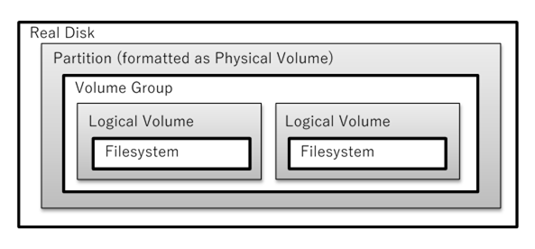
Note growing/shrinking an LV is a separate operation from growing/shrinking the filesystem within that LV. (There are exceptions.) Also, not all filesystems types support growing and/or shrinking at all. (XFS only supports growing.) In those cases, you need to backup the files to an appropriate type of backup or archive, create a new filesystem in the resized LV, then restore the files. NTFS must be defragmented before shrinking; ext* can be resized anytime with resize2fs.

LVs have a number of parameters that can be set (and most can be changed later) that can affect disk I/O performance, including extent size, chunk size, stripe size, stripe set size, and read-ahead.

LVM is complex to setup (and varies among Unixes) but is compatible with hardware RAID, and implements software RAID. Note that if / (root) is a LV, then you must have a non-LV /boot as it is the BIOS that finds boot loaders, and BIOS doesn’t understand about LVM.

LVM Snapshots [from LVM-HOWTO at tldp.org]

One of the features you get with LVM is a snapshot. This allows an administrator to create a new logical volume which is an exact copy of an existing logical volume (called the original), frozen at some point in time. This copy is usually read-only (although read-write is possible; see rollback below). A common use includes when a backup needs to be performed on the logical volume, but you don’t want to halt a live system that is changing the data. Another use is just performing some system maintenance; if that doesn’t work out, you can rollback the system to the snapshot. (If it does work out, you can easily find and diff all the files that were changed.)

When done with the snapshot, the system administrator can just unmount it and then remove it. This facility does require that the snapshot be made at a time when the data on the logical volume is in a consistent state, but the time the original LV must be off-line is much less than a normal backup would take to complete.

In addition, the copy typically only needs about 20% or less of the disk space of the original. Essentially, when the snapshot is made nothing is copied. However, as the original changes, the updated disk blocks are first copied to the snapshot disk area before the original LV is written with the changes. The more changes are made to the original, the more disk space the snapshot will need. This type of snapshot is known as a COW (copy on write).

When creating logical volumes to be used for snapshots, you must specify the chunk size. This is the size of the data block copied from the original to the snapshot volume. For good performance this should be set to the size of the data blocks written by the applications using the original volume. While this chunk size is independent of both the extent size and the stripe size (if striping is used), it is likely that the disk block (or cluster or page) size, the stripe size, and the chunk size should all be the same. Note the chunk size must be a power of 2 (like the stripe size), between 4K and 1M. (The extent size should be a multiple of this size.)

You should remove snapshot volumes as soon as you are finished with them, because they take a copy of all data written to the original volume and this can hurt performance. In addition, if the snapshot volume fills up errors will occur.

Red Hat made a utility to create and manage snapshots for BtrFS or LVM, called snapper.

Rolling Back a Snapshot From evms.sourceforge.net

Situations can arise where a user wants to restore the original volume to the saved state of the snapshot. This action is called a rollback. One such scenario is if the data on the original is lost or corrupted. Snapshot rollback acts as a quick backup and restore mechanism, and allows the user to avoid a lengthier restore operation from tapes or other archives.

Another situation where rollback can be particularly useful is when you are testing new software. Before you install a new software package, create a writeable snapshot of the target volume. You can then install the software to the snapshot volume instead of to the original, and then test and verify the new software on the snapshot. If the testing is successful, you can then roll back the snapshot to the original and effectively install the software on the regular system. If there is a problem during the testing, you can simply delete the snapshot without harming the original volume.

You can perform a rollback when the following conditions are met:

· Both the snapshot and original volumes are unmounted and otherwise not in use.

· There is only a single snapshot of an original. (If an original has multiple snapshots, all but the desired snapshot must be deleted before rollback can take place.

Example of Snapshot Creation and Rollback

# lvcreate -L 1G -n lv_test vg
# mkfs -t ext4 /dev/mapper/vg-lv_test
# mkdir /test /snap
# mount /dev/mapper/vg-lv_test /test
# echo hello > /test/foo
# lvcreate -s /dev/mapper/vg-lv_test -L 1G -n snap
# echo goodbye > /test/bar
# mount /dev/mapper/vg-snap /snap
# ls /test
bar foo lost+found
# ls /snap
foo lost+found
# umount /test
# umount /snap
# lvconvert --merge /dev/mapper/vg-snap
# mount /dev/mapper/vg-lv_test
# ls /test
foo lost+found

LVM (and ZFS) Tips [from sun.com/bigadmin/features/articles/zfs_overview.jsp]

· A small number of storage pools (or volume groups) with many disks works better than a large number of small pools/VGs.

· Use whole disks not partitions.

· Try to have DB data use one controller and DB indexes use another.

· ZFS filesystems aren’t a limited resource. You can create as many of these as you want. One thing you must avoid is splitting the root filesystem as this will prevent live upgrade from working. You might have one filesystem for each Zone, projects get their own, and anything that benefits from different filesystem properties get their own. A good example of the latter is media requiring an uncompressed filesystem. You can also split backups: low volume but important data can be sent off-site, bulk data to a local mirror.

· With lots of ZFS filesystem, to make a snapshot for backups, there is a recursive option so you don’t need to make separate snapshots of each one. (LVM doesn’t have such an option currently.)

· ZFS filesystems inherit properties from their parent ZFS filesystem. So you can make a change to the parent and all the children will pick it up automatically.

Storage, even for a simple single server, has become complex. You have LVM and device-mapper (dm), encrypted disks, software RAID (multiple disks, or MD), and newer filesystem types that incorporate these concepts such as BtrFS and ZFS.

Red Hat created a command line tool that can work with all these storage technologies, known as System Storage Manager (SSM), or system-storage-manager. By using a single user interface and multiple back-ends for the different technologies involved, SSM can make managing your storage easier.

Choosing a type of Filesystem

This depends on how it will be used. Not all filesystems can dynamically grow and/or shrink. Not all support ACLs, quotas, attributes or extended attributes (needed for SE Linux). Some favor speed over reliability (in the event of an unexpected system failure, not all filesystems recover well) or reliability over speed. Some support large numbers of small files better, or small numbers of large files better. Some include more utilities than others; UFS (BSD) and ext2/3/4 (Linux) include dump and restore utilities for backup and recovery, fsck for system integrity checking and repair, tunefs (tune2fs) to examine and change filesystem settings, and other tools to resize a filesystem or to defrag one. On the other hand, some systems include no backup/restore utilities, no tools to change parameters after filesystem creation, and in some cases, no fsck tool.

Use the fstyp command on Solaris (non-x86) to determine the filesystem type of some disk (or partition). For Linux and some others, use “file -s /dev/sda” and/or “parted -l /dev/sda”.

Modern Filesystem types use journaling to eliminate need for fsck after a power failure (only!). ext4 is safest of these, ReiserFS, XFS require a UPS to be safe but are much faster, especially with lots of smaller files. JFS2 works well for larger (>16-256GB, the limit for ext3) files, ok for smaller ones, and is safer than XFS or ReiserFS. (Note the Linux file size limit of 2TB regardless of FS type, and can be further restricted from the shell using ulimit.)

With journaling, a filesystem records the commands for changes to a log (or journal) file. Only after that has been written safely and completely will they make the change to the filesystem. Once the data has been safely and completely updated, they remove that journal entry. If the system crashes at any point, it can simply replay the journal entries to restore the system. This works because of a property of such journal entries: they are idempotent. That means, running such commands more than once won’t corrupt anything.

Solaris 10 on x86 supports most common filesystem types. You may need to install additional software packages to use them: FSWpart and FSWfsmisc. To mount such filesystems, you need to learn the device name and filesystem type for each partition on each disk. The prtpart x86 tool shows this information. (Solaris fdisk doesn’t work well for DOS disks.) The mount command needs the FS type; Solaris names these pcfs, ntfs, and ext2fs (ext2, ext3, and ext4). All but DOS (pcfs) are currently supported as read-only.

Journaling filesystems depend on the journal entries being written in the correct order. But in order to increase benchmark numbers most disk drives have on-board caching and use disk write reordering. Experiments have shown that there is a 1 out of 10 chance of filesystem corruption after an uncontrolled shutdown. Linux kernel places write barriers at intervals to prevent such corruption, but if possible, data write reordering should be turned off (hdparm -W 0) when using a journaling filesystem. Using RAID striping makes this situation worse as stripes can become inconsistent.

Most journaling filesystems only use the journal for metadata, not the contents of files. If the system crashes while writing a large file to disk, the journal will make sure the hard link and block counts are correct, but you still only have half a file; the data is corrupted. Ext3 and ext4 are unusual because they journal all data (by default; you can change that). However, this hurts performance.

Remember, a filesystem is not a database! “File systems are optimized very differently from data bases. Databases have transactions that can be committed or rolled back if the database or the application decides to abort a transaction. In contrast, file systems do not support the concept of rollback or undo logs, and one of the reasons for this is in order to get very high performance levels, ...” [Ted Ts’o blog post].

Ext3 and ext4 are most suited to non-server, commodity PCs. Servers using RAID and UPSes may choose a type for performance over protection. Recently some mobile devices switched to ext4 (e.g., android). This has caused a problem with some applications (e.g., Firefox) which frequently update various databases on every mouse click (awesome bar), causing annoying delays.

Other filesystem types commonly used include vfat (pcfs on Solaris; matches nearly all Microsoft FAT filesystem types, and ntfs matches NTFS) for small flash drives and floppies, and iso9660 (hsfs=high sierra on Solaris) for data CD-ROMs, and udf is the successor to iso9660, used on DVDs and flash drives >32GB (the max for the FAT flash drives use standard). See mkisofs, growisofs, cdrecord (run 1st with -scanbus to get device number triplet; only supports SCSI so must use IDA-SCSI adopter modules) (Solaris: cdrtool), and mkdosfs. Linux supports JFFS2 and UBIFS, and LogFS for flash drives; MS has exFAT (a.k.a. FAT64); there are others too.

Without a UPS, when the power fails not all parts of the computer stop functioning at the same time. As the voltage starts dropping on the +5 and +12 volt rails, certain parts of the system may last longer than other parts. For example, the DMA controller, hard drive controller, and hard drive unit may continue functioning for several hundred of milliseconds, long after the DIMMs, which are very voltage sensitive, have gone crazy and are returning total random garbage. If this happens while the filesystem is writing critical sections of the filesystem metadata, you can corrupt the FS beyond hope of recovery. Ext3 [and ext4] is designed to be recoverable in this situation; other, higher performance FSes are not. — adopted from Ted T’So, linuxmafia.com/faq/Filesystems/reiserfs.html

(Point out wikipedia.org/wiki/Comparison_of_file_systems article.)

UFS is the modern version of the BSD FFS (1983). A UFS volume is composed of the following parts:

· a few blocks at the beginning of the partition reserved for boot blocks (which must be initialized separately from the filesystem).

· a superblock, containing a magic number identifying this as a UFS filesystem, and some other vital numbers describing this filesystem’s geometry and statistics and behavioral tuning parameters.

· a collection of cylinder groups. All data for a directory and its contents are kept (if possible) on one group, minimizing fragmentation. Each cylinder group has the following components:

o a backup copy of the superblock

o a cylinder group header, with statistics, free lists, etc, about this cylinder group, similar to those in the superblock

o a number of inodes, each containing file attributes

o a number of data blocks

UFS was so popular it was adopted by most Unix vendors, who sadly made many incompatible changes to the basic idea. Among the ideas were the inode structure.

Inodes (for modern UFS and similar FS types) store 15 pointers to data blocks in an inode; the first 12 point directly to data, the 13-th is an indirect block (the whole block contains pointers to data blocks), the 14-th is a doubly indirect block, and the 15-th is a triply indirect block. This is not efficient for large files.

EXT2 is fastest since it doesn’t use journaling but is very reliable. Recovery can be slow (tens of minutes to hours per filesystem, depending on size and speed of hardware). It is based on the original “ext” FS from 1992, which in turn was based on Minix FS, which was based on BSD’s UFS. This is a 32-bit FS which limits max size. Ext2 FSes can be grown or shrunk as needed.

EXT3 is a tweaked version of ext2. The major change was to add journaling. (In fact, it is easy to convert ext2 to ext3 and vice-versa.) Unlike most FSes that provide journaling, ext3 journals all writes to disk, not just “metadata” (inode and directory writes). This provides more reliability than other journaling FSes but slows down data writes.

An SA can control what gets journaled with a setting (using tune2fs). Set “data=journal” for journaling everything. Set “data=writeback” to just journal metadata. Use the default of “data=ordered” to improve performance while providing almost at much safety as for “journal” mode. With this option the FS will write data to the disk (as a transaction) after making the journal entry for the affected metadata, but before writing the metadata itself.

EXT4 is based on ext3. It uses 48-bit addresses rather than 32-bit. It also changes the way large files are managed. Instead of the UFS inode pointer structure, the idea of “extents”, first used with JFS and later with XFS and NTFS among others) provides better performance for large files, such as those used with DBMSes. Overall, ext4 is faster than ext3 but just as reliable.

(Ext4 originally didn’t support the ext3 “data=ordered” mode (see above), but Ted Ts’o reluctantly added this back.)

An extent-based filesystem doesn’t allocate space for files a block at a time, but in large variable-sized chunks called extents. Inodes contain a list of pointers to extent descriptor blocks, organized as a B-Tree for fast access.

JFS was one of the first journaling filesystems. It was developed by IBM for AIX Unix in 2001. Unlike ext* this is a 64-bit FS designed for high performance servers. It differs from traditional *nix filesystems by allowing several independent disk writes to be collected and committed as a one large “group” transition; fewer transactions means fewer journal updates and better performance. Small directory data can be saved directly in the inode itself (if it will fit), causing half as many disk accesses. Large directories are not a simple list but have directory entries organized as a “B+ Tree”, a data structure that can be searched efficiently. Another difference is the inode table isn’t fixed in size when the FS is created, but rather inodes are allocated as needed. JFS FSes can be grown but not shrunk. JFS also supports different block sizes on a per-file basis.

XFS was developed by SGI (Silicon Graphics, Inc.) for IRIX (a popular Unix in the ‘90s). In many ways it is similar to JFS. XFS is highly scalable, high-performance file system. It was created to support file systems up to 16 exabytes (approximately 16 million terabytes), files up to 8 exabytes (approximately 8 million terabytes) and directory structures containing tens of millions of entries. XFS supports metadata journaling, which facilitates quicker crash recovery. XFS file system can also be defragmented and expanded while mounted and active; it is not possible to shrink XFS file system.

XFS is popular with NAS systems or large enterprise storage systems. Red Hat Enterprise Linux 7 (along with Fedora) uses XFS as the default FS (previously, EXT4); it is also the only choice for RH’s Storage offerings. (SuSE also has used XFS for years as the default, but recently switched to BtrFS.) XFS is considered a mature product with high-quality code and active development (by Linux kernel developers; independent development seems to have stopped around 2013), however XFS lacks many of the features and tools of ext4.

Red Hat’s switch to XFS in 2015 was surprising, but “it’s a better match for our enterprise customers” stated Denise Dumas, Director of Software Engineering for Red Hat. As for SuSE, they say they preferred XFS over Ext4 “due to concerns about scalability as the tools package only recently supported file systems in excess of 16TB. Ext4 also suffers from issues that require applications to be updated and make use of fsync calls to guarantee data is committed to disk.” While I don’t think those are valid reasons today (2016), another reason is that the author and maintainer of ext4 recommends BtrFS.

ReiserFS (a.k.a. Reiser3 FS) Reiser4 FS are highly innovated journaling filesystems with many, many performance improvements. However, it lacks the reliability of other FS types. Once considering promising, the lead developer was convicted of murder in 2008 and the future of this FS type is uncertain.

Other types supported on Linux include MSDOS (for FAT16), VFAT (for FAT32; pcfs on Solaris), NTFS, iso9660 (hsfs on Solaris), UDF (used on data DVDs and large Flash disks), NFS, and SMBFS (networking filesystems), and special purpose FSes such as GVFS, or those for cluster use (GFS, GPFS).

When real-world applications grow beyond what a single server can provide, you either need to scale-up (a.k.a. vertical scale) by using a more powerful server, or scale-out (a.k.a. horizontal scale) by using a cluster of cheap servers. With a cluster, a load-balancer of some sort distributes work to the various servers. However, a customer session may be composed of many interactions with a server. Some interactions will be sent to one server, others to a different server.

To meet such needs, you either need network attached storage (the storage is on one server and the cluster servers read/write to it), or a distributed filesystem. There are many of these, each with different properties (so you need to match the filesystem to the application’s use of files). Some commonly used distributed filesystems include HDFS (used with Hadoop), GFS (developed by Google), GFS2 (by Red Hat), GlusterFS, and Ceph (very popular).

BtrFS (“Butter FS” or perhaps “better FS”) has features comparable to Sun’s ZFS. It is being actively developed by Oracle (and others). While available since 2010, adoption is slow (2017). Theodore Ts’o has stated that ext4 is a stop-gap and that Btrfs is the way forward, having “a number of the same design ideas that reiser3/4 had”.

Theodore Ts’o (the primary developer of ext2/3/4) suggested, “People who really like reiser4 might want to take a look at btrfs; it has a number of the same design ideas that reiser3/4 had — except (a) the filesystem format has support for some advanced features that are designed to leapfrog ZFS, (b) the maintainer is not a crazy man and works well with other [Linux] developers (free hint: if your code needs to be reviewed to get in, and reviewers are scarce; don’t insult and abuse the volunteer reviewers as Hans did — Not a good plan!).” kerneltrap.org/mailarchive/linux-kernel/2008/8/1/2780064

SuSE, who for many years advocated XFS, now uses BtrFS as the default. “It works with Snapper to implement snapshot and rollback, the killer function of Btrfs. You can pick any date you saved to rollback your full system” said George Shi. Fedora 33 Workstation also uses BtrFS as the default (but not Fedora Server).

In addition to performance (for large numbers of small files or a small number of large files), reliability (journaling metadata and/or file data), and max size, there are other differences between filesystem types: if an FS can grow or shrink, support for POSIX data (owner, group, permissions (mode), etc.), support for attributes, for extended attributes, for NFSv4 attributes/permissions, for MAC security (e.g., SE Linux) labels, support on various OSes, built-in LVM/RAID features, snap-shot and rollback support, disk scrubbing, and quota support. How important these features are depends on the expected use of the file system.

BetrFS The Be-tree File System (pronounced “better eff ess”) should not be confused with BtrFS! It is a newer (2020) FS that claims much improved performance over ext4, zfs, and btrfs.

ZFS is Sun’s open sourced newest FS and is available for Linux and other Unix systems too. (Note to self: make a web resource). The name originally stood for Zettabyte File System but is no longer considered an acronym for anything. The name was a misnomer since ZFS can manage 256 quadrillion zettabytes (10^33) but there is no SI unit prefix for that. (The only higher prefix is yotta, 10^24.) ZFS is a complete redesign of filesystem concepts and includes LVM and RAID built-in, as well as automatic mounting, growing and shrinking as needed, and nested filesystems. It is very scalable, supporting very large files and directories. It also includes disk scrubbing, a sort of continuous fsck.

Simple ZFS commands replace many LVM and other commands (mount, mkfs, ...) [June 2006 issue of Login; has ZFS article.]

ZFS organizes physical devices into logical pools called storage pools. Storage pools can be sets of disks striped together with no redundancy (RAID 0), mirrored disks (RAID 1), striped mirror sets (RAID 1 + 0), or striped with parity (RAID-Z, really RAID 5). (See below for a full description of RAID.) Additional disks can be added to pools at any time, but they must be added with the same RAID level as the pool was created with. As disks are added to pools, the additional storage is automatically used from that point forward.

ZFS file systems will grow (to the size of their storage pools) automatically. If you define more than one ZFS file system in a single pool, each shares access to all the unused space in the pool. As any one file system uses space, that space is reserved for that file system until the space is released back to the pool by removing file(s). (You can place a maximum size on a filesystem, confusingly called a quota.

ZFS file systems are not necessarily managed in the /etc/vfstab file. Special logical device files can be constructed on ZFS pools and mounted using vfstab, but the common way to mount a ZFS file system is to simply define it against a pool. All defined ZFS file systems automatically mount at boot time unless configured not to.

The default mount point for a ZFS file system is based on the name of the pool and the name of the file system. For example, a file system named data1 in pool indexes would mount as /indexes/data1 by default. This default can be overridden.

Use the format command to determine the list of available devices, then create a pool with: zpool create pool-name [configuration] device-file ...

Where configuration may be mirror, raidz, etc. Once created a default ZFS FS is created and mounted as /pool-name. To change FS parameters or to create additional FSes in the pool, use the zfs command:

# zfs create pool-name fs-name

To monitor your pools, use zpool list. Likewise use zfs list (or mount). Other monitoring sub-commands are also useful.

Please refer to the man pages, zfs(1M) and zpool(1M), for more detailed information. Additional documentation may be found at oracle.com/technetwork/indexes/documentation/index.html#sys_sw (formerly docs.sun.com). Another resource is the OpenSolaris ZFS Community.

[from: sun.com/bigadmin/features/articles/zfs_part1.scalable.jsp]

ZFS is a combination of file system and volume manager; the file system-level commands require no concept of the underlying physical disks because of storage pool virtualization (i.e., LVM). ZFS is a journaling FS that uses transactions to modify the data. All of the transactions are atomic so data is never left in an inconsistent state.

ZFS only performs copy-on-write (COW) operations. This means that the blocks containing the in-use data on disk are never modified. The changed information is written to new blocks; the block pointer to the in-use data is only changed once the write transactions are complete. That disk block is then also updated via COW. This happens all the way up the file system block structure to the top block, called the uberblock.

(In terms of memory, COW means something different: processes will share a single copy of a memory page until one of them writes to that page, at which point the copy is made.)

If the machine were to suffer a power outage in the middle of a data write, no corruption occurs because the pointer to the “good” data is not moved until the entire write is complete. (Note: The pointer to the data is the only thing that is moved.) This eliminates the need for journaling data blocks, and any need for fsck (or mirror resync) when a machine reboots unexpectedly. (Ext4 journals all data; ZFS, ReiserFS, and others that only journal some data aren’t as safe, but are faster.)

To avoid accidental data corruption, ZFS provides memory-based end-to-end check-summing. Most check-summing file systems only protect against bit rot because they use self-consistent blocks where the checksum is stored with the block itself. In this case, no external checking is done to verify validity. This won’t catch things like:

· Phantom writes where the write is dropped on the floor

· Misdirected reads or writes where the disk accesses the wrong block

· DMA parity errors between the array and server memory or from the driver, since the checksum validates the data inside the array

· Driver errors where the data winds up in wrong buffer inside the kernel

· Accidental overwrites such as swapping to a live file system

With ZFS the checksum is not stored in the block but next to the pointer to the block, all the way up to the uberblock. Only the uberblock has a self-validating SHA-256 checksum. All block checksums are done in server memory, so any error up the tree is caught including the aforementioned misdirected reads and writes, parity errors, phantom writes, and so on.

In the past, the burden on the CPU would have bogged down the machine, but these days CPU technology and speed are advanced enough to check disk transactions on the fly. Not only does ZFS catch these problems, but in a mirrored or RAID-Z (Really ZFS RAID-5) configuration the data is self-healing. One of the favorite Sun demonstrations showcasing data self-healing is the following use of dd where c0t1d0s5 is one half of a mirror or a RAID-Z file system:

dd if=/dev/urandom of=/dev/dsk/c0t1d0s5 bs=1024 count=100000

This writes garbage on half of the mirror, but when those blocks are accessed, ZFS performs a checksum and recognizes that the data is bad. ZFS then checksums the other copy of the data, finds it to be valid, and resilvers the bad block on the corrupted side of the mirror instead of panicking because of data corruption.

In a RAID-Z configuration, ZFS sequentially checks for the block on each disk and compares the parity checksum until it finds a match. When a match is found, ZFS knows it’s found a block of valid data and fixes all other bad disks. The resilvering process is completely transparent to the user who never even realizes that a problem had occurred.

ZFS constantly checks for corrupt data in the background via a process called scrubbing. The administrator can also force a check of an entire storage pool by running the command zpool scrub. This should be done via cron 1-2 times a month.

A DBMS such as MySQL or PostgreSQL can be implemented on ZFS and eliminate redundant journaling, data validation, atomic writes, etc.

Fedora 11 made BtrFS (“Butter FS” or “Better FS”) available as a technology preview. To enable BtrFS, you had to pass icantbelieveitsnotbtr as a boot option.

ZFS vs Btrfs vs Stratis

ZFS is open source, but under a different license than Linux: CDDL vs GPL. The two are not compatible, making it risky for vendors to include ZFS with Linux. Btrfs is close (or as close as it will get) to feature-parity with ZFS and is available in a compatible license. However, Btrfs is controlled mainly by Oracle and Red Hat has decided to no longer support it. Instead, they launched their own storage solution, Stratis. See Red Hat’s docs for Stratis for more.

Oracle could just relicense ZFS but have refused to do so. So for Linux, you have ext4 or Btrfs as your main choices.

RHEL 8 uses Stratis. This offers nearly the same features as Btrfs, but is actually a front-end for XFS, LVM, and other technologies. Apparently, Red Had decided Stratis would be cheaper in the long run, as other groups maintain the individual technologies used. (If RH adopted Btrfs, they would need to maintain it.)

(Due to limitations of XFS, I personally prefer to continue with LVM + ext4.)

Lecture 5 — Storage (Disk) and Related Technology

The Storage Hierarchy [From queue.acm.org "Flash Today" , by Adam Leventhal, September 24, 2008]

Primary storage can be summarized as a unit of storage, or more precisely as controller containing CPUs and DRAM, and attached to disk drives. The disks are the primary repository for data while some memory (DRAM) acts as a very fast cache. Client software communicates with the storage via read and write operations. Read operations are always synchronous in that the client is blocked until the operation is serviced, whereas write operations may be either synchronous or asynchronous. For example, video streams may write data blocks asynchronously and verify only at the end of the stream that all data has been quiesced; databases typically use synchronous writes to ensure that every transaction has been committed to stable storage.

The speed of a synchronous write is limited by the latency of nonvolatile storage, as writes must be committed before they can be acknowledged. Read operations first check in the DRAM cache, which can provide fast service times. But cache misses must also wait for the disk. Since it’s common to have working sets larger than the amount of cache available, even the best prefetching algorithms (a technique to anticipate the next read and fetch it into the cache) will leave many read operations blocked on the disk.

The common technique today to reduce latency is to use 15,000-RPM drives rather than 10,000-, 7,200-, or 5,600-RPM drives. This will improve both read and write latency, but only by a factor of two or so. This can be pricey. For example, a 10-TB data set on a 7,200-RPM drive (from a major vendor, at 2008 prices) would cost about $3,000 and dissipate 112 watts; the same data set on a 15,000-RPM drive would cost $22,000 and dissipate 473 watts. The additional cost and power overhead make this an unsatisfying solution.

A better way to improve the performance of synchronous writes is to add NVRAM (nonvolatile RAM) in the form of battery-backed DRAM, usually on a PCI card. Writes are committed to this NVRAM ring buffer and immediately acknowledged to the client, while the data is asynchronously written out to the drives. This technique allows for a tremendous improvement for synchronous writes, but NVRAM is expensive, batteries can fail (or leak or even explode), and the maximum practical size of NVRAM buffers tends to be small (2-4 GB)—small enough that workloads can fill the entire ring buffer before it can be flushed to disk.

This is where using flash memory for an NVRAM ring buffer is becoming popular. However, while achieving good write bandwidth is fairly easy, the physics of flash dictate that individual writes exhibit relatively high latency. It’s possible, however, to insert a small DRAM write cache on top of the NVRAM buffer, treating it as nonvolatile by adding a capacitor that in case of power loss provides the necessary power to flush outstanding data in the DRAM to the flash cache.

Hard Disks

(Show hardware graphic: Spindles, platters (aluminum or glass), heads.) Sectors and cylinders (tracks) and heads (platter faces) = disk geometry (“CHS”). Discuss speed (5,400–15,000 rpm; seek time). Each read/write chunk is one sector (512 bytes on all disks up to 2011; starting in 2011 all disks have 4096-byte sectors). (Cylinder/track 0 is the outermost one on any magnetic disk.)

One block (a.k.a. a cluster) is smallest chunk of disk that can be allocated by the OS to a file, so one block is smallest file size. On Sun systems (UFS) a block is 512 bytes (1 sector) of data, on Linux (ext[23]) it is 1024. (On Reiser4FS it is 1 byte!)

The 512-byte sector size dates from the earliest IBM floppy disk standards. But there are problems with this size. Newer disks use weaker signals to record the data, so more parity bits are needed per sector. Currently (2010) each 512-byte sector has 40 bytes reserved for the low-level formatting “start of sector” mark, and 40 bytes reserved for parity. (Prior to 2004 only 25 parity bytes were needed.)

New disks use 4096 (8 “old” sectors) byte sectors. This greatly reduces the overhead, even though the new disks will use 100 bytes per sector for parity.

Using 4kB sectors will make many operations faster and take less power. This is because the logical block/cluster size for NTFS and some other filesystems is also 4kB. Also, on x86 processors the page size of memory is 4 KiB. So, most disk operations are already 4 KiB.

Most newer BIOSes (and EFI) can support the new sector size and new OSes can too. Note that Windows XP won’t support the new disks! Western Digital will ship disks with an “emulation mode” to support older firmware and OSes. In this mode performance may suffer. It would probably be better to use a virtual machine for WinXP. (From MS: “... [Microsoft] strongly cautions against using 512e media with Windows XP. 512e media are the latest Advanced Format (AF) drives with an emulation layer that creates two different sector sizes. While the system may boot up and be able to minimally operate, there may be unknown scenarios of functionality issues, data loss, or sub-optimal performance.

The IDEMA has mandated the change starting in 2011. It wouldn’t hurt to stock-pile some older type disks if you need them!

Unformatted Capacity Versus Usable Capacity

Disks are sold by their total unformatted capacity. Both low-level and high-level formatting a disk takes a significant fraction of that space, as does the spare sector list (used for mapping out bad sectors), boot code, hidden or reserved areas on the disk, RAID and LVM metadata, etc. Since most filesystems use blocks (or clusters) to allocate files, a file of size 1 block plus one byte takes two blocks of disk space. With many small files the usable space can be less than half the unformatted capacity. For example, I have a 1GB flash drive with the standard FAT FS on it. After formatting there are 977 MB available. I put about 200 small files on it, leaving about 700 MB reported free. However, I couldn’t put even one more file on it!

Some OSes allow you to adjust the block size in some filesystems to reduce wastage (but reduces I/O speed.) Others permit packing multiple file fragments into blocks.

Disk Geometry and LBA (Logical Block Addressing)

The number of sectors per track varies with the radius of the track on the platter. The outermost tracks are larger and can hold more sectors than the inner ones. The location of sectors is staggered as well, for efficiency.

But disk geometry is just a triple: #cylinders, #heads, #sectors (“CHS”). The growth of disk sizes means modern disks must lie about their true geometry. Rather than use CHS addressing it is common to use a Logical Block Addresses (LBA mode), in which each sector is given a number starting from zero. The OS uses LBA rather than CHS addresses, which is then translated by the disk to the actual sector.

Some OSes use BIOS to access disks (which is also used at power up), and (older) BIOS uses CHS addressing. So BIOS must know the official (but fake) geometry setting. (Even then the disk must translate the official geometry to the real geometry!) Others OSes directly access disks with LBAs and don’t care.

Prior to LBA the combined limitations of BIOS and ATA restricted the useful unformatted capacity of IDE hard disks on IA PCs to 504 megabytes (528 million bytes):

1024 cyls * 16 heads (tracks/cyl) * 63 sectors/track * 512 bytes/sector

Later BIOSes and ATA disks use LBA mode to work around those limits, by faking the geometry and translating to the official one. (This still leaves a BIOS disk size limit of 1024 cylinders * 63 sectors per track * 256 heads * 512 bytes per sector = 8 gigabytes; such older BIOS can’t boot from a partition beyond the first 8 GBs.) This is one motivation for the modern BIOS replacements (e.g., EFI).

Modern OSes (including Windows and Linux) are not affected by this since these OSes use direct LBA-based calls and do not use BIOS hard disk services. Also modern BIOSes support larger disks and LBA. Older BIOS limits affect booting: /boot below cylinder 1024. (LBA needs to change for 2011, for the 4kB sectors.)

Shingled disks (SMR, shingled magnetic recording) are used for very large HDDs, those over 2 TB in size. SMR disks overlap tracks like shingles on a house, hence the name. SMRs can only write large blocks called bands at a time, maybe 30 MiB. To change a single disk block requires reading the whole band into RAM, making the change there, then writing the whole band back. (This is similar to how SSDs work.) Because of this, random writes are expensive (slow). This affects everything when using a journaling filesystem such as ext4, which writes small metadata blocks to the journal all the time. (Changes to ext4 to make it SMR-aware are being proposed as of 5/2017 (“ext4-lazy”).

Before purchasing SMR disks, be aware of the negative performance effects.

Hard disks are not reliable. They fail frequently. A 2007 Google study of 100,000 hard drives showed the average annual failure rate was 6% (1 in 20). Only 25% of the disks survived 5 years or more. Similar studies confirm these numbers. Manufacturers quote MTBF (mean time between failures) numbers that are not realistic.

RAM Disks

RAM disks (a.k.a. “ramdisks”) are a technique to use a part of memory as if it were a disk. Programs on your system think they are reading and writing files to an ext4-like filesystem, but the data stays in memory. Why do this?

There are many reasons: speed was a major reason, but ramdisks are rarely used anymore just for speed since the Unix virtual memory system is so efficient. Instead they are used for initial booting, for /tmp on Solaris and other OSes, for security, to mount (potentially a large number of) disk image files, and only occasionally for efficiency. (Not all software can be rewritten to use memory when they were designed to use files, but you can use a ramdisk in such cases.)

RAM disks are a section of memory that is used as a filesystem (and thus that RAM is not available for other purposes). These can be used to speed access to programs and other files, used while booting, or to check a disk. A ramdisk can double the battery life on a laptop! Many servers need to create many short-lived files quickly (such as PHP session files) and a ramdisk is the best choice for that.

All systems support at least one ramdisk driver (or type); Linux supports several, some for special purposes. For example, you will see a ramdisk mounted at /dev/shm for POSIX shared memory.

Modern Linux supports several types of ramdisks: the old “ramfs” which uses physical memory, and the newer “tmpfs” which uses both swap and RAM. This is mostly useful for /tmp. It can also be used to hold security-sensitive documents that shouldn’t be written to actual disk. Note you don’t format ramfs or tmpfs filesystems! While not ext4, they behave similarly.

Linux since 2014 supports zram, a ramdisk block device (unformatted) that can be used for any purpose, for example, swap. The zram driver uses fast compression (I think the “z” is for “zip”) and provides high performance while taking less memory than other types of ram disks. (Note this is unrelated to zero-capacitor zram, except for the name.) Use of zram is becoming popular (2019). See the kernel’s zram docs for usage and other info.

The main difference between ramfs and tmpfs are that ramfs uses physical RAM only and if that runs out your system can crash. Tmpfs uses virtual RAM (so it can use swap space as needed). Also tmpfs allows you to specify a maximum size to which the RAM disk is allowed to grow.

By itself, a ramdisk is useful for temporary data files. In some cases, you want to save the contents of a ramdisk to a file and restore the state of that ramdisk from a file when mounting it. Such a file is usually called a disk image file. This ramdisk plus image file technique is used during the boot process.

Modern Linux includes a kernel-created variation of tmpfs called devtmpfs. The kernel creates this very early at kernel initialization, before any device drivers are loaded. Every detected device that has a driver in the kernel will have a device node created in this tmpfs instance, even before the device is initialized. Then the devtmpfs is mounted at /dev.

Unix and Linux can mount an image file as if it were a disk. This is similar to using a ramdisk and copying an image file to/from it, but more convenient.

An initial ramdisk is often needed during the boot process. This is initialized from an image file. It is used as an initial root filesystem and contains some required /dev files, /lib files, init, etc.

(SSDs, or solid-state disks, are discussed below.)

Creating RAM disks is easy. (For Solaris: “ramdiskadm -a mydisk 40m” will create /dev/ramdisk/mydisk, which you must format and then mount as normal.) To create and use a ramdisk on Linux (note no formatting needed!):

# mkdir /mnt/ramdisk
# mount -t ramfs none /mnt/ramdisk # Old

# mount -t tmpfs size=32m /mnt/ramdisk # New
# cd /mnt/ramdisk; vi foo; ...
# cd; umount /mnt/ramdisk

Live CDs and other image files must often be compressed to fit the image on the media. A common technique is to use “squashFS” compression. If the file command shows some image file type as this, use “unsquashfs image” to uncompress it; then file will show the correct type (you need to know the type to mount it).

(Linux also has a block ramdisk driver; with that, you would need to run mkfs on it before you could mount it.)

The RAM disk starts out small and grows as needed. With tmpfs you can optionally specify a maximum size. This is a good thing to do since if a system runs out of virtual memory, ugly things will happen!

When a ramdisk is unmounted (via umount), all files in it are lost.

You can specify a max size with tmpfs, with the mount option size=size (the default is half the size of physical RAM). The size is in bytes but you can add a k, m, or g suffix. You can also specify a max number of inodes with nr_inodes=number. (The default is half the number of physical RAM pages.)

On Solaris, you can use a RAM disk for a RAID 1 mirror. This can be useful if an application is mostly reading from the disk. In this case you can change the read policy for the mirror to first read from the RAM disk.

More common than a real ramdisk is to mount an image file (.img, .iso) using a loop device. A “jukebox” can be created by putting many image files on a large disk and mount them all. (Project 4, filesystems, discusses how to use image files.)

Historical note: Linux creates some fixed-size ramdisks at boot time:

ls -l /dev/ram*; dmesg | grep -i ram

shows the system creates 16 4K RAM disks. To set the size use the kernel (boot) parameter ramdisk_size=sizeInBytes. Unlike ramfs/tmpfs these are not initialized. Before you can mount one of these you need to format it with mkfs.

If planning on using ramdisks (say for /tmp) you will need a larger swap partition (and possibly more RAM) then the standard guidelines suggest.

Solid State Disks (SSD) — Flash Memory

This is a newer technology that is increasingly used. It’s just a large amount of non-volatile RAM and works like a USB flash disk. As it gets popular and/or cheaper, there will be many changes to how storage is managed: no seek time issues, different block sizes, etc. (Of course, there will be other issues!) (There’s a good article on SSDs available at Ars Technica.) As of 2017, SSDs costs about 5 times as much per GiB as HDDs, so it will be a while before regular disks are “legacy technology”. (Show Nand flash SSD image.)

Why should you care about the technology behind SSDs? Solid state drives have two problems that force them to deal with data differently than hard disk drives do: they can erase data only in larger chunks than they can write it, and their storage cells can only be written a certain number of times before they start to fail. This number is reported a program/erase cycles per cell, or P/E cycles. 10,000 for TLC and 100,000 for SLC are typical numbers for 2021. A company called Greenliant sells NAND SSDs that promise up to 250,000 P/E cycles as of 4/2020. This makes tasks such as modifying files much harder for SSDs than HDDs. (See “endurance” below for more info.) Thus, setup, failure modes, monitoring, and tuning are all different.

Flash memory can be implemented using either NAND or NOR logic. These designations that refer to the way the flash cells are arranged. NOR flash allows for random access and is best suited for random access memory, while NAND must be treated as blocks and is better for persistent storage. NAND flash is cheaper and by far the more common variety. (I am unaware of any commercial NOR flash SSDs available today, although NOR flash is used in a variety of products.)

There are different types of NAND flash (2018): SLC (single-level cell), MLC (multilevel cell, which means two levels), and TLC (triple-level cell). SLC stores a single binary value in each memory cell, using one voltage level for “0” and another for “1”. MLC supports four voltage level values per memory cell, corresponding to two bits of storage. TLC supports 8 voltage levels and thus 3 bits per cell.)

Because of its improved longevity, performance, and reliability, SLC is best suited for enterprise (i.e., non-consumer-grade) solutions; because of its low price, MLC / TLC (which wear out the cells several times faster; typical writes per cell is 3,000 as opposed to 10,000 for SLC) is common for consumer-grade SSDs; TLC is cheapest to manufacture. MLC/TLC has higher error rates than SLC and are generally slower. Today there is also eMLC (enterprise grade MLC) with lower error rates, but it is also slower than SLC.

NAND Flash disks are fast to read (0.25 ms access time, compared to 8 ms for hard disks). Random reads are more than 100 times faster than for hard disks (Sequential reads are more than twice as fast as for hard disks).

Writing to flash is harder; data is written in blocks (pages or rows) of 512 to 4,096 bytes, which must be erased before each write. (Bit can be flipped from 1 to 0, but you must erase the whole block to set a single bit back to a 1!) Each block has a short lifetime as well; SLC flash is typically rated to sustain thousands of program/erase cycles per block. For a busy server, that doesn’t seem like much, however you might get 5-10 years from such an SSD.

Another distinction is that NOR flash can access individual bits in each block of data. NAND flash can only access whole rows (pages) at a time in a block. This results in a lot less wiring for NAND, making the devices less than half the size of the same amount of storage implemented using NOR.

Cells in NAND flash memory are arranged in rectangular grids known as blocks. A typical block may have a million cells or so. The rows of the blocks are the addressable units of storage; only whole rows can be read/written at a time. A row in a block is also called a page.

A typical NAND flash memory grid (block) has 32 to 256 columns (cells) per row (page), and 4,096 to 65,536 rows. (In practice, the pages are a little larger to include error-correction and bookkeeping data.) Each block thus stores between 16 KiB to 2 MiB (512 KiB is common).

The blocks are grouped into planes. Each plane might hold 1,024 blocks. A single NAND flash chip contains one or more planes; each plane can do operations in parallel with outher planes (or whole chips; depends on the controller). An SSD is made up of many chips, a controller, and a RAM cache. Show SSD card image. See also Flash NAND array image.

NAND memory can only be read or written a page at a time. Also, you can only write to an erased page. Pages cannot be individually erased. Only whole blocks can be erased.

It takes about 1-2 ms to erase a block, but writing to an erased flash page requires only around 200-300 µs (that’s .2-.3 ms). For this reason, flash devices try to maintain a pool of previously erased blocks so that the latency of a write is just that of the program operation. Read operations are much faster: about 25 µs (that’s .025 ms) for 4k. By comparison, raw DRAM is even faster, able to perform reads and writes in much less than a microsecond; HDD access is about twice as slow. To deal with data arriving faster than it can be written, consumer-grade SSDs contain some DDR2 or faster SDRAM used as a cache, usually between 128 and 512 MB.

To rewrite a small file (say using vi) a solid-state drive has to copy everything on the block (say, 512KB), except for the deleted data, to memory, then erase the entire 512KB block the file is in, and finally rewrite all of it again along with the new version of the file. In SSD circles, this is called garbage collection: recognizing that a file is old and invalid, removing it, and rewriting it with good data (many drives will collect little files in their RAM to modify and write in big chunks, but the idea is the same). Such garbage collection significantly reduces the speed SSDs are known for, because reading, modifying, and rewriting is much slower than a simple write. Also, the SSD doesn’t recognize deleted files (only the OS and it’s filesystem driver are aware) and continuously rewrites them during this garbage collection process.

A new SSD command, TRIM for ATA and UNMAP for SCSI, can be sent by the OS to help an SSD recognize deleted files. There is a mount option called discard to send these commands whenever a block is freed. However, there is a performance penalty for doing so and many people prefer to schedule the Linux fstrim command to run once a week.

(Windows since 8 will issue TRIM when defragmenting SSDs (ref) if the optimize option is on). You can also use the Windows defrag.exe command manually.)

Fedora since 32 schedules fstrim weekly.

Garbage collection and other activities mean that SSDs are constantly moving data around, writing twice as much as you might guess, and wearing out the drive sooner than you might think.

This design makes SSDs work differently than hard disks (HDs). When new, SSDs are full of empty pages and seem speedy. As they age, they run out of empty pages and must do garbage collection, which slows them down noticeably. This also means that until the device gets nearly full, all old versions of data are still there; overwriting a file with zeros (as with a HD) won’t generally overwrite the file! A HD over-writes old data with new data (an in-place update). with SSDs you need to use TRIM.

Modern SSDs support “secure erase”, which restores the drive to original factory state, and restores performance.

For example, in current-generation (2020) SSDs with 8192-byte pages, a block can be made up of as many as 256 separate pages (2 MiB), meaning that to write an 8KiB file, the SSD must actually first copy two mebibytes of data into cache, then erase the whole block, then re-write most or all of the entire 2 MiB.

As flash cells are used, they lose their ability to record and retain values. As mentioned above, each cell can be erased and written 3 to 10 thousand times before failing. Because of the limited lifetime, flash devices must take care to ensure that cells are stressed uniformly so that “hot” (frequently used) cells don’t cause premature device failure. This is done through a process known as wear leveling (or write-leveling). Just as disk drives keep a pool of spare sectors on each track for bad-block remapping, flash devices typically present themselves to the operating system as significantly smaller than the amount of raw flash, to maintain a reserve of spare blocks (and pre-erased blocks for performance).

Wear-leveling has security implications: you can’t guarantee data has been erased when the cell holding that data may have been duplicated before the erase. Most flash devices are also capable of estimating their own remaining lifetimes so systems can anticipate failure and take action to protect the remaining good blocks.

Wear-leveling and the need to erase blocks before writing means data is moved about and written multiple times. This phenomenon is known as write amplification and can cause SSDs to wear out faster than many benchmarks indicate.

The cache works just like one on a HD and has the same issue of data reported as written once in the cache, so a power failure results in data corruption. The better SSDs have a large capacitor that can power the cache long enough to transfer the data to the non-volatile SSD. (Enterprise SSDs don’t have that, apparently because of an assumption of high-quality UPSs in data centers.)

Another issue to be aware of: the cells of SSDs may not fall on logical disk block boundaries. If they don’t match when formatting the SSD, each read/write of a disk block will require two reads or writes per block! This issue is called partition alignment, and most partitioning tools will handle this correctly, but some may require the sys admin specify options to align the partition disk blocks on cell boundaries (typically, 4 KiB).

The final issue is data loss. Like HDDs, SSDs will lose data if powered off for too long. Enterprise SLC SSD drives stored at 25C and operated at 40C have a typical retention rate of just 20 weeks without power. In worst-case scenarios or high storage temps, the data on an enterprise drive can start to fail within seven days. (HDDs usually retain data for 1-2 years in this scenario.)

Flash storage costs about $1-$20 per gigabyte for an SLC flash device compared with around $50 per gigabyte for DRAM (as of 2018). Disk drives are still much cheaper than flash, about $0.02 per gigabyte for 7200-RPM drives and under $1 per gigabyte for 15,000-RPM drives. (Checked prices 2/2018 from NewEgg and Amazon.)

From a Slashdot post on 2013-12-27: “After the reports on SSD reliability and after experiencing a costly 50% failure rate on over 200 remote-deployed OCZ Vertex SSDs, a degree of paranoia set in where I work. I was asked to carry out SSD analysis with some very specific criteria: budget below £100, size greater than 16Gbytes and Power-loss protection mandatory. This was almost an impossible task: after months of searching the shortlist was very short indeed. There was only one drive that survived the torturing: The Intel S3500. After more than 6,500 power-cycles over several days of heavy sustained random writes, not a single byte of data was lost. Crucial M4: failed. Toshiba THNSNH060GCS: failed. Innodisk 3MP SATA Slim: failed. OCZ: failed hard. Only the end-of-life’d Intel 320 and its newer replacement, the S3500, survived unscathed. The conclusion: if you care about data even when power could be unreliable, only buy Intel SSDs.

Recent flash disks have improved on all fronts: smarter/faster controllers, 2 or more times the number of write (P/E) cycles, and lower costs. Most SSD drives are guaranteed to last 3 years (for lowest grade drives) to over 10 years for enterprise grade drives. That’s just the guarantee; the drives will likely last many times longer than that.

Reliability is a function of the spacing of NAND cells. The closer they are packed, the less reliable the device. 3D NAND or Vertical NAND (V-NAND) flash improve reliability by spacing the cells farther apart, but have multiple layers of such cells (the cells are stacked vertically on the chip, to be taller but take less area).

For example, the Intel Optane 3D X Point or the Samsung 850 EVO are faster, take less power, and have a longer life than 2-D SSDs. (See X Point, below.) Samsung introduced the 24-layer V-NAND in 2013, 32-layer V-NAND in 2014, 48-layer V-NAND in 2015, 64-layer V-NAND in 2016, 9x-layer V-NAND in 2016, and 1xx-layer V-NAND in 2019, allowing terabyte-sized but still reliable SSDs. Virtually all modern SSDs use V-NAND to stack multiple layers of NAND flash.

A hybrid approach is somewhat common: using an SSD as a cache for a regular HDD. Support for this is known as bcache in Linux.

An SSD needs a more sophisticated controller than a simple USB flash drive, to deal with management of pages and blocks, the complexities of writing, RAID-0 like data stripping (plus some parity), wear leveling, multiple I/O channels (to access the different chips in parallel), managing the SDRAM cache, garbage collection, and other tasks.

SSD lifetime, commonly known as endurance, is generally specified either in Drive Writes per Day (DW/D or DWPD) or Terabytes Written (TBW). These numbers represent the amount of user data the device is guaranteed to be able to write over the device’s lifetime. Drive Writes per Day is the most common measurement used to express an SSDs endurance specification. This number, which can vary from under 0.1 to over 10, indicates the amount of data that can be written each day for the warranty period. For example, a 1TB SSD with 3 DW/D and a warranty of 5 years should allow for writes of 1TB * 3 DW/D * (365 * 5) = ~5.5PB. Note the capacity of the drive can greatly affect endurance, so be careful when comparing drives.

The lifespan of consumer grade SSDs continues to improve. It is likely that a modern (made after 2014) SSD will outlast the PC it is installed on. But for servers and their heavier loads, SSDs will often lose their speed advantage, not last longer than HDs, and cost more. In 2018, newer technology promises faster/longer/cheaper, but we will have to wait to see if that is so.

Defragmenting Filesystems and SSDs

All filesystems write new files to contiguous blocks on the storage device. However, over time files get deleted leaving “holes”. Sooner or later, new data must be stored in those holes, resulting in the new files being fragmented.

Fragmentation hurts performance in two ways. Each fragment must be read using a separate disk READ operation (only contiguous blocks can be read in a single IOP). There is overhead for each disk I/O operation (IOP). Secondly, for HDDs each READ may result in a disk seek which is very slow. Even if the fragments are on the same cylinder, other processes are issuing disk IOPs and those may end up being done between your process’ IOPs. Thus, two or more seeks may occur between those reads! The slower reads (and writes too) will be noticeable on large data reads such as for backups or loading huge software/data into memory.

Defragmenting flash storage is rarely necessary and wears out the device fasting by performing unnecessary writes. However, defragmenting can improve performance on SSDs, just not as dramatically as for HDDs. Modern defragmenting tools are SSD-aware, and will issue TRIM/UNMAP commands when run, which definitely will improve performance. (Including for Windows 8.x and newer.) Note that some defrag tools attempt to coalesce the free space into one large block at the end of the drive (pointless on SSDs) while other merely try to reduce the number of fragments per file (still useful on SSDs).

For NTFS, there is also the problem of hitting the max number of fragments for the filesystem. Without regular defragmenting, an NTFS volume can become full and/or corrupted!

Finally, fragmented filesystems require defragmenting before certain operations are performed, such as resizing them.

While the jury is still out on this issue (2017), recent research shows SSDs do suffer some performance loss when fragmented. Unlike HDDs, this effect has nothing to do with physical placement of file blocks. Rather, fragments cause more disk I/O operations (the OS can only issue single I/O requests for contiguous blocks). That and a lack of regular TRIM/UNMAP commands can cause about a 25% performance slow-down in the worst case reported. (HDDs suffer over 200% slow-downs when badly fragmented.)

Since modern SSD units can last for billions of writes, an occasional defragmenting (say 1/month) shouldn’t hurt. But don’t expect dramatic performance increases, unless you’ve used the drive for years and have never run a tool on it (thus, not TRIM/UNMAPs or secure erase).

There are many places in current computers and operating systems that assume HDs and thus are not correctly configured for SSDs. The following are some Windows 10 settings to change (in 2018), from an article in Admin. Many of these points should be double-checked on Linux systems as well:

· To make optimal use of SSDs, enable Advanced Host Configuration Interface (AHCI) mode in the BIOS/UEFI. This requires the correct drive is installed and enabled, which you can check on with Device Manager.

· Many people claim that users should deactivate the paging file on SSDs. This is not a good idea.

· You can obtain an overview as to whether the SSD and the rest of the hardware are working properly. To do so, start the metric by typing winsat formal or winsat prepop at the command prompt. Toward the bottom of the list you will see the read and write speeds of the SSD.

· AS SSD Benchmark freeware is very helpful when determining SSD performance. Well-known comparison websites, such as Tom’s Hardware use the tool to compare disks. (The home site is in German; try FileHippo’s site for English.)

·       One problem when mirroring (copying) Windows 10 to an SSD (from a HD) is the relationship between the start of the boot partition and the storage blocks of the hard drive (alignment). This problem occurs whenever you move the operating system from a magnetic hard drive to an SSD instead of installing from scratch. If the start of the boot partition and storage blocks do not match, SSD performance is compromised and its lifespan shortened: The boot partition, rather than starting at the beginning of a sector, begins in the middle, because the filesystem clusters do not match the SSD pages. To check, call for the StartingOffset data on the command line:
          wmic partition get name, startingoffset
Then, call the filesystem data of the corresponding hard disk:
           fsutil fsinfo ntfsinfo c:
Check the Bytes Per Cluster value: You have to divide the StartingOffset value by the Bytes Per Cluster. The result has to be a whole number. If this is not the case, you should consider reinstalling Windows 10 on the SSD.

·       TRIM also plays an important role in the use of SSDs. If you delete files from your system, their data remains on the hard disk and is only deleted from the file allocation table (or inode table). The actual file data is still stored on the hard drive. The OS overwrites this data when the operating system needs the space.
Data deletion does not work the same way on SSDs. The storage blocks must be completely deleted first before they can be rewritten. Windows 10 supports the TRIM technology and tells the SSD which storage blocks it can delete. However, many current SSDs come with technologies that internally delete storage blocks via the controller and the internal firmware, and thus tell the OS not to use TRIM.
You can check TRIM support in Windows 10 by entering
           fsutil behavior query DisableDeleteNotify
If you see DisableDeleteNotify=0, then TRIM is supported, whereas DisableDeleteNotify=1 indicates deactivation. With the command
           fsutil behavior set disablenotify 0
you can enable TRIM in Windows 10.

· To improve the performance of SSDs, you should always install the latest firmware on the device. If the manufacturer makes a new version, you should download and install it, then reboot your PC.

· Some Windows tools enable automatic defragmentation of boot files during startup. This doesn’t give you any noticeable performance improvements with normal hard disks, but it is actually harmful for SSDs, which is why you should disable the feature. Open the registration editor (regedit), navigate to HKEY_LOCAL_MACHINE | SOFTWARE | Microsoft | Drfg | BootOptimizeFunction, and set the OptimizeComplete value to No to disable the function.

· The Windows memory manager SuperFetch determines user behavior and immediately optimizes memory so that frequently used applications are temporarily stored in RAM and available quickly. The technology can also distinguish behavior through time; thus, it is possible for office applications to be optimized during office hours and leisure programs or games to be optimized during the weekend. However, this function no longer makes sense with SSDs and puts a strain on the hard disk. Windows 10 automatically disables this service when installing on an SSD, but you should check if it is enabled from services. You can also disable the SuperFetch and Prefetch functions in the registry by opening the registry editor, navigating to the HKEY_LOCAL_MACHINE | SYSTEM | CurrentControlSet | Control | Session Manager | Memory Management PrefetchParameters entry, and setting the EnablePrefetcher and EnableSuperfetch values to 0.

· Because SSDs consume less power than magnetic hard drives, an energy-saving mode is of little value for SSDs. Therefore, you can adjust the energy settings of your OS to support SSDs by leaving the hard disk enabled.

· Because of TRIM technology, you have to be careful when restoring deleted files. With normal hard disks, files marked as deleted can be overwritten immediately without doing anything to the data in those files. However, SSDs and other flash memory devices do not work this way: The controller truly has to delete existing data that are no longer needed. Controllers normally run these processes if a certain memory area is idle, which means that on SSDs and flash drives, it is possible a deleted file has in fact been completely removed, and not just its entry in the filesystem’s allocation table. On top of that, if the file hasn’t been deleted there may be multiple versions of it in different blocks. Thus, special tools are needed for data recovery from SSDs. Recuva (from the makers of the popular ccleaner tool) is the most popular Windows tool for recovering data on SSDs and flash drives.

3D XPoint Memory

3D XPoint is a new kind of persistent (non-volatile) solid state memory devised by Intel and Micron. Limited commercial releases are available (2017), known as Intel Optane. Details on how the memory actually works are not publicly released (yet). The cells in the blocks are manufactured in three dimensions: rows (pages) are made up of columns of stacks of cells. This new memory is byte addressable; you can read/write bytes at a time, same as RAM. It can also be used as SSD. Because of the high density of the chips, 3D XPoint is much cheaper than DRAM.

The performance is not as good as fast RAM, but close enough for many use cases and much better than flash technology. The performance is designed for “big data” applications: 3D XPoint has about one thousandth the latency of NAND flash (which has 10x the latency of DRAM), and can be manufactured tens of times the density of DRAM, allowing for an impressive amount of memory (terabytes instead of gigabytes) that can sustain a large number of I/O operations/second “IOPS”).

Erasing 3D XPoint memory blocks wears them out 3 to 60 times less rapidly as flash NAND cells, so the devices last longer. Since this is just the first generation of this new technology, I expect the performance to improve and the cost to decrease over time. Non-volatile RAM will be a game-changer; you won’t need traditional storage as much. (See image of Micron 3D NAND Flash.)

Directly Attached Storage (DAS)

This used to mean the disks were inside the computer enclosure. Today’s servers are small form-factor rack-mounted servers or blade servers. In either case the disks are not enclosed by the computer. With DAS you are limited to having the disks in the same cabinet. With DAS the disk attaches to an interface (e.g., SCSI). A cable connects that to a host interface (the controller), which usually allows more than one disk to be attached to the host computer.

DAS is also used for RAID devices to attach several disks to a special RAID controller. This in turn is attached to the host computer as if it were a simple disk.

The Future: It has been predicted in 2016 that fast, non-volatile memory may make all storage technology obsolete (and require re-designing operating systems and programs). The technology exists now (3D X Point), but the price is high.

Disk Controllers

There are two common types of disk controllers: IDE (or EIDE or ATA), used with SATA, and SCSI. The controllers support many options (we’ll learn some of these later). One option to know about now is a write cache, which should be turned off for reliability. However, leaving it on (the usual default) dramatically increases performance.

Solaris provides the tool fwflash(1M) to examine and load (or flash) firmware on some models of HBAs (which are sometimes referred to as host channel adaptors, or HCAs).

IDE/ATA

Allows two devices per IDE controller (technically called a channel), referred to as the controller and the other the worker (even though neither controls the other). It is common to have two controllers per workstation, referred to as the primary and secondary. ATA disks must be within 18" of their controller, so sometimes the controller is connected to a host with a cable to an HBA (Host Bus Adaptor; see below).

IDE became EIDE then ATA (Advanced Technology Attachment, a.k.a. PATA, ATAPI, and UDMA) to support CD-ROM and other devices. Not as fast (~133Mbps) or reliable as SCSI, but cheaper. 18" cable max length, so it’s good only for DAS. The controller is usually integrated into the motherboard. To date (2021) there have been 9 versions of the ATA standard (plus some unofficial ones and the newer SATA standards).

AT (since v3) allows sneaky commands to permit the disk to hide some space from the OS, using a Host Protected Area (HPA) and Device Configuration Overlay (DCO). Actually, at boot time the OS can access the HPA then lock it down so Microsoft can hide stuff there. The HPA and DCO are hard but not impossible to access, with special software.

Serial ATA

(SATA or S-ATA) is the successor to IDE, which was retroactively renamed Parallel ATA (PATA) to distinguish it from Serial ATA. ~300Mbps, more than double the speed of the older IDE (parallel ATA) disks (but slower than SAS). Modern workstations use SATA. The cables are much smaller (versus the 40+ pin ribbon cable), and can be 1 meter in length (versus 18"). To the OS, each disk appears as the main on a separate IDE controller. (I.e. one disk per controller.)

With older hardware, parallel cables were faster since you could send 8 (or more) bits simultaneously, compared to serial (where you might also need extra bits sent to control timing). But with modern electronics, the speed that data is sent is much higher. Parallel wires generate interference, putting a limit on the top speed they can use. Serial cables are now capable of higher speeds than a parallel cable, are cheaper, and easier to work with.

SATA drives are geared mostly toward end-user systems, not servers. Then tend to try to automatically fix any detected errors (which can cause delays that cause software or OS time-outs). For use in RAID systems, you want the drive to report errors as quickly as possible, so the data can be fetched from another device in the RAID set. Write caches may be unreliable, and advanced control commands (e.g., to flush the cache) may be ignored. Also, firmware tends to be upgraded fairly often even on the same model drive; thus it may be impossible to replace one bad disk. (There is such a thing as enterprise (or RAID) grade SATA drives, but these are much more expensive.)

There are other differences between SCSI and SATA, including some marketing ones (vendors use SCSI for their higher-grade products). Generally however, SATA is as fast and as reliable as SCSI today. SATA disks are generally “consumer grade”, usually 5400 to 7200 RPMs (some are available up to 10,000 RPMs), and come in very large capacities.

The 6 Gib/Sec limit of the SATA bus was plenty for HDs, but not fast enough for SSDs. Today there is SATA Express, using the same physical connector as SATA but using PCI Express lanes to boost speed. An x2 (two lanes) SSD is faster than the 6 Gib/Sec of SATA, and you can use 4x or more.

For SFF (small form factor) and similar devices, a different bus, M.2 is becoming (2015) common. Like SATA Express, it uses PCI Express lanes.

SCSI

A SCSI device includes a “controller” that talks to the system’s SCSI bus controller. (That makes SCSI disks more expensive than ATA ones.) The system SCSI controller is slightly misnamed, as it is only a bridge connecting the SCSI bus to the host bus; it passes commands and results between the CPU and the SCSI devices. (A system SCSI controller is sometimes also known as a host bus adaptor, or HBA.)

The SCSI bus can connect disks or any similar devices: CD-ROM, DVD, Tape, etc. These devices are peers on the bus, just like with Ethernet NICs. SCSI disks are mostly considered “enterprise grade”, although it’s notable that Macintosh computers have always used SCSI. Today you are likely to use Serial Attached SCSI or SAS. (Discussed later.)

Compared to the disks usually sold with SATA controllers, these disks generally have smaller capacities but are much faster, often 15,000 RPMs. The drivers report errors quickly, which is needed for RAID use. The firmware tends to be more stable too, making it likely you can replace a failed disk someday with a compatible one. However, all that speed and reliability comes at a price; SCSI is more expensive than ATA disks.

The SCSI controller is physically part of the disk so you purchase, unlike ATA disks which do require an extra controller per disk. This helps makes SCSI disks more expensive than ATA disks. With SANs, the actual SCSI disks may be far away, and a special type of NIC called an “HBA” is used to talk to them.

With some manufacturers, the same physical disk can be used with either ATA or SCSI controllers. You merely change the drive enclosure (which contains the controller electronics).

With IDE/EIDE/ATA/ATAPI, the device driver sends commands to the controller, which sends AT (ATAPI is “ATA Packet Interface”) commands to the disk (by loading data registers, then sending a signal). In contrast, with SCSI the device driver sends SCSI commands directly to the device (disk). The SCSI controller or HBA simply forwards those commands onto the bus (and sends any reply back to the device driver).

Many devices (8 to >95) can be daisy-chained together, with the end of the chain needing termination. The electrical specifications for a SCSI bus require each end of the bus to be properly terminated. You must use the appropriate type of terminator for your bus; passive, HVD or LVD. If the controller is controlling only an internal bus or only an external bus, it will usually provide termination either automatically or via BIOS configuration.

Although ATA disks must attach to the host with a cable no more than 18", the total length of the SCSI daisy-chain is 1.5 meters (UltraSCSI), 3 meters (FastSCSI), 6 meters (old SCSI), 12 meters (low-voltage differential, or LVD SCSI), and 25 meters (high voltage differential, or HVD). If your disks are further away from the host than those limits, you must use some remote storage technology.

If you mix wide and narrow devices on one SCSI bus, be aware that the termination for narrow devices may occur in a different place to the termination for wide devices.

SCSI IDs

Each device is assigned a unique SCSI-ID (or SCSI address), with the controller usually assigned ID 7. (The boot disk usually gets ID 0.) Older, “narrow” SCSI has 8 IDs (0–7), while “wide” SCSI has 16 (0–15). These IDs may be set automatically or manually. You may have to manually assign SCSI-IDs to avoid conflicts!

Devices on a SCSI bus have a priority. The higher IDs have higher priority. The extra 8 IDs for wide SCSI all have lower priority than 0. So the priority order of IDs is: 8 (lowest), 9, 10, 11, 12, 13, 14, 15, 0, 1, 2, 3, 4, 5, 6, 7 (highest). Devices that cannot tolerate delays (such as CD or DVD recorders) or slower devices (such as tape drives) need high priority IDs to ensure they get sufficient service.

Devices such as RAID controllers may present a single ID to the bus but may incorporate several disks. In addition to the ID, the SCSI addressing allows a Logical Unit Number or LUN. Tapes and single disk drives either do not report a LUN, or report a LUN of 0.

A SCSI adapter may support more than one SCSI cable or channel, and there may be multiple SCSI adapters in a system. The full ID of a device therefore consists of an adapter number, a channel number, a device ID, and a LUN.

Devices such as CD recorders using IDE-SCSI emulation and USB storage devices will also appear to have their own adapter.

SCSI LUNs:

A SCSI device can have up to 8 ‘sub-devices’ contained within itself. (Some SCSI busses support more than this: 32, 128, or even 254.)

The most common example is a RAID controller (single SCSI ID) with each disk (or more commonly a logical volume) in the array assigned a different LUN. Another example is a CD-ROM jukebox that handles more than one disk at a time. Each CD/DVD is addressed as a LUN of that device. Most devices (such as hard disks) contain only one drive and get assigned LUN zero. Some of these devices internally ignore LUNs and if queried will report the same device for any LUN. Beware of auto-detection!

Each unique controller.channel.scsi-id.lun gets a device in /dev. On Linux, disks will be named /dev/sd?, tape drives will be /dev/st#, and CD and DVD drives will be /dev/sr# (deprecated) or /dev/scd#.

Example: a software RAID of two disks will appear as /dev/sda (the RAID’s logical device), /dev/sdb and /dev/sdc (the disks within the array). Usually you only access /dev/sda, but may need to access the others to re-mirror or to get status. Of course, if using hardware RAID, you won’t see the sub-devices at all on your system.

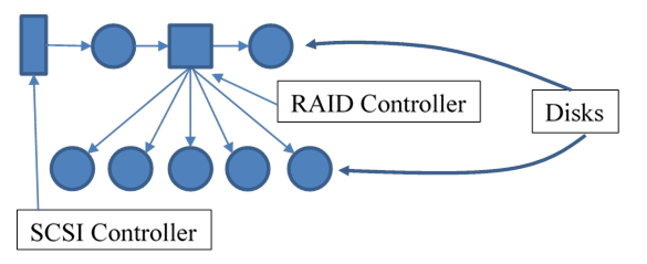
(In this diagram, the devices in the top row get SCSI IDs; those in the bottom row get LUNs.)

All SCSI devices regardless of type get assigned /dev/sg# as well. You can use the Linux sg_map command to see which devices correspond to the generic ones.

Note: A RAID controller plugs into the SCSI chain and the disks plug into the RAID controller’s internal bus, which may or may not be SCSI (so as to use cheaper ATA disks). The RAID controller usually won’t report the LUNs to the SCSI driver in your kernel.

Linux provides a large number of commands to query and control SCSI devices, all starting with “sg”. Try (as root) “sginfo device”.

SCSI Types

SCSI is faster, more flexible, and more expandable than IDE and is used almost universally on servers, but usually is considered too expensive for workstations. Note that a disk must have the correct connectors as well as the correct on-board software to talk to an HBA (often called the controller).

SCSI is very fast (>300Mbps), reliable, and allows longer cables than IDE. There are several incompatible SCSI standards in use today. The devices/connectors are marked with different symbols (SE, LVD, and DIFF) but it is up to you to not mix incompatible ones (some devices may be marked as SE/LVD which can use either). (Mixing types can cause serious damage and risk electrical fire!) Types:

SCSI-1 8-bit bus, 5MBps, bulky Centronics connector.

SCSI-2 Same as SCSI-1 but with Micro-D 50 pin connector.

Fast 8-bit bus, 10MBps, Micro-D 68 pin connector.

Ultra 8-bit bus, 20MBps, Micro-D 50 pin connector.

Ultra2 8-bit bus, 40MBps, Micro-D 50 pin connector

Ultra3 (a.k.a. Ultra-160) 8-bit bus, up to 160MBps

Ultra-320 320MBps

Ultra-640 (a.k.a. fast-320) 640MBps but limited cable length, # devices

Wide 16-bit bus, 10MBps (same clock rate as SCSI-1), Micro-D 68 pin connector

There are also fast wide, ultra-wide (a.k.a. SCSI-3), wide ultra2, ...

iSCSI Ultra-3 SCSI but using TCP/IP and Ethernet for the bus.

Serial SCS and other new developments: not really SCSI but uses SCSI command set to communicate with devices.

Although many of these busses support high speed by default, the clock rate will automatically adjust down to the speed of the slowest device on the bus. So use 2 controllers (1 for slower tape/CDROM, one for fast disks). You can manually set the speed to adjust for longer than normal cable lengths or flaky devices.

Controller Protocol Example: SCSI Commands

An OS must use a controller’s protocol to tell it what to do. In SCSI terminology, communication takes place between an initiator (typically the host) and a target (typically one of the disks). The initiator sends a command to the target which then responds. SCSI commands consist of a one-byte operation code followed by five or more bytes containing command-specific parameters. At the end of the command sequence the target returns a Status Code byte which is usually 00h for success, 02h for an error (called a Check Condition), or 08h for busy.

There are 4 types of SCSI commands: N (non-data), W (writing data from initiator to target), R (reading data), and B (bidirectional). There are about 60 different SCSI commands in total. (AT commands are simpler.) Here are a few:

· Test unit ready - “ping” the device to see if it responds

· Inquiry - return basic device information

· Request sense - give any error codes from the previous command

· Send diagnostic and Receive diagnostic results - run a simple self-test, or a specialized test defined in a diagnostic page

· Start/Stop unit

· Read capacity - return storage capacity

· Read

· Write

In all cases (both DAS and remote storage) the older parallel interfaces (P-ATA) are going away in favor of serial cables and interfaces. The reasons are simple: parallel cables are bulky, expensive, slower, and have greater distance limitations than serial cables.

Newer Storage Controller Standards

Consumer computers today (2016) mostly use SATA (with SCSI commands). The standard protocol between the system and disk controllers is AHCI (Adv. Host Controller Interface). However, these are inadequate for SSDs; server hardware tends to use proprietary protocols. SATA v3.3 (the current standard, 2017) can only support 500 IOPS (I/O operations per second) and 600 MBps, under ideal conditions. SSDs could operate at 20,000 IOPS today, and prototypes have been shown to use 2 million IOPS.

The SATA working group decided they’ve reached nearly the limit of SATA, and suggested newer computers switch to newer buses and protocols. Currently, PCIe (PCI express) is recommended as it can support up to 1 GBps, and can use multiple parallel “lanes” (2x, 4x, etc.).

There’s still the limit of AHCI though; it cannot take full advantage of PCIe. For modern SSDs a newer standard is needed.

NVMe (non-volatile memory express) replaces AHCI and other solutions such as SATA and SAS (where a controller plugs into PCIe and the SSD plugs into the controller). Modern SSDs simply plug into PCIe slots, but needed proprietary drivers to talk to the disk. NVMe is an open standard for this use. (NVMe is really the next generation of PCIe.) There is considerable industry support for NVMe; many consumer PCs have it now (2020).

RAID

RAID (Redundant Array of Inexpensive Disks; since modern disks are not inexpensive some have claimed the “I” means “independent) is a technique of using multiple disks to improve performance, fault tolerance, or both. It is a fact of life that disks, whatever technology is used, sometimes fail. Often the failure is just some bad data (data written ≠ data read), other times whole blocks become unreliable and must be avoided, and sometimes the entire disk dies. RAID fault tolerance helps keep the system up in these cases, avoiding a service interruption to restore from a backup (and the associated data loss).

Each RAID level defines some combination of striping, replication, and parity. Striping means to write logically consecutive sectors to different disks, which speeds things up. Replication or mirroring makes multiple copies of data on different disks. Parity data allows the RAID controller can detect when some disk contains corrupted data; with enough parity data the controller can determine which disk is bad. The system can continue by using the remaining good disk(s).

[ Uses Flash: www.acnc.com/raid.html; uses animated GIFs: lascon.co.uk ]

RAID Level	Description
0	*striping* — Spread data over disks fast reads and writes, poor reliability
1	*mirror* — duplicate data on 2 or more disks. (*Duplex* means mirror with one controller per disk.) Requires OS support. fast reads, good reliability, very expensive
0+1 (01)	mirror of RAID 0 sets reliability and costs of RAID 1 with faster reads; rarely used
1+0 (10)	striping across RAID 1 sets same as 0+1 but more reliable; best for production databases
2, 3, 4	striping + parity (slight variations in type of parity) cheaper than mirroring with similar reliability. Slower performance due to dedicated parity disk
5	striping + (distributed) parity can survive any one disk failure with degraded performance, otherwise performance of striping (not quite) with reliability of mirroring but cheaper. Most popular.
6	striping + (distributed) parity (More parity than RAID 5) can survive any two disk failures, with degraded performance. Popular for larger RAID systems such as for SANs.

Most level number definitions vary. Only RAID levels 0, 1, 1+0, 5, and 6 are standard. All these extra disks can be expensive! Low-cost servers may have just two (identical) disks and can opt for striping (performance) or mirroring (safety). With four disks you can stripe across mirrored sets, or mirror each strip set.

Parity data used for standard RAID is known as n+1 parity. Each bit of each byte of each block of the data disks (there may be more than two) are XOR-ed to produce parity bits (except for RAID 2). For example, assume RAID 3 (stripe+parity): Disk1Block1byte1 = “1011 0010”, D2B1b1 = “1100 1111”, then P1B1b1 is “0111 1101”. If a disk fails, the data can be recalculated from the others. For example if D2 fails: D2B1b1 = D1B1b1 XOR PB1b1 = 1011 0010 XOR 0111 1101 = 1100 1111.

Needing X out of Y data blocks to reconstruct a file of Y blocks is called erasure coding. RAID 6 is “4 + 6” (four of six) scheme. With large data sets, distributed across several data centers, RAID mirrors are common for reliability. Erasure coding provides the same reliability with far fewer disks, useful if a hurricane takes out one of your data centers. However, there is an additional computational overhead, and thus latency, with this scheme.

RAID can be supported in either hardware or software. (Note, your book omits duplexing from definition of RAID1.) Software RAID >0 will impact performance. (RAID 5 in software can be about 23% slower!)

As noted previously, some modern filesystems (ZFS, Btrfs) provide per-block integrity checks, a process called disk scrubbing. The OS in this case computes a checksum of each disk block, stored elsewhere on the disk. In the background, the OS continuously recomputes these and compares with the stored version, to detect any discrepancies. This process is not a substitute for RAID parity.

Be careful to avoid “fake” hardware RAID controllers! If the controller is labeled as “software” or “host” RAID, it is not a real hardware RAID controller; it uses your computer’s CPU and memory rather than its own. (This is similar to “win-modems” and “win-printers”.) Good, real controllers are made by LSI, 3ware (purchased by LSI), Areca, Adaptec, Intel, and HighPoint. Some controllers are re-branded ones such as Dell PowerEdge (really LSI). To tell the difference, you can compare the price of several “real” controllers and if you see an unknown model for substantially less money, it is likely software RAID. Also, the manufacturers of hardware RAID cards/controllers will document the specifications in some detail on their web sites. If you can’t find a detailed specification for some RAID card, get a different one. Another way to tell is if they offer an option to add onboard battery-backed memory to the card; only real RAID has onboard cache. Always check the specifications; even “real” RAID controllers can be low-quality.

If a disk in a RAID set (using mirroring) fails and you replace it, the replacement process will put a lot of load on the remaining disk(s) which may then fail due to the excess load!

Using RAID storage systems in a data center (with SAN or NAS), it pays to have huge disks. The RAID system then defines logical volumes and assigns each a LUN. This is done in a vendor-specific way but efforts are underway to create a usable open standard for this (SNIA’s RAID disk data format, or DDF). Different servers are assigned different LUNs. The OS sees each LUN as a disk to be partitioned and formatted.

The Linux software RAID driver is called “md” (multi-device); see mdadm and consider turning off mdmonitor if not using software RAID. See also mdmpd. On Debian, see mkraid. On Solaris, metainit, metattach. Note most hardware RAID controllers are incompatible with SMART device monitoring; you’d have to access the individual disks and not all RAID controllers make that possible. (However, many such controllers do SMART health checks for you and have some other way to show any issues.)

Replacing a bad disk from a hardware RAID set:

Nearly all servers have status lights on the disks, although they may not always indicate a failure. Usually. you can determine which is the failed disk, by examining the logs which report the /dev/disk/by-path/ bus/SCSI notation (Solaris: /dev/dsk/cXtXdX notation), then find the matching entry from the output of the RAID controller software. (Show ls /dev/disk/by-path.)

Running Red Hat on HP Proliants merely need to look for the failed drive with the bright red light on, rip it out and stick a new one in. This is picked up by the hardware RAID controller and the operating system never even notices!

On Solaris, you must look at the output of “cfgadm -la” and run:
“cfgadm -c unconfigure matching_disk_entry”. This will shut the drive down and trip the LED indicator. Once the drive is replaced with a good one, run:
“cfgadm -c configure matching_disk_entry”. (Depending on your system (e.g., Sunfire) you run the Solaris luxadm command instead.)

Software RAID (Linux) Example: A RAID 1 array formatted with ext4:

# mdadm --create /dev/md0 --level=raid1 \
--raid-devices=2 /dev/sda1 /dev/sdb1
# mkfs -t ext4 /dev/md0

The mdadm configuration file tells an mdadm process running in monitor mode how to manage hot spares, so that they’re ready to replace any failed disk in any mirror. See spare groups in the mdadm man page. (Note you could do this with LVM instead. LVM uses the md driver under the hood.)

The startup and shutdown scripts are easy to create. The startup script simply assembles each mirrored pair RAID 1, assembles each RAID 0 and starts an mdadm monitor process. The shutdown script stops the mdadm monitor, stops the RAID 0s and, finally, stops the mirrors.

As mentioned previously, modern disks aren’t as reliable as many believe. A study (Data corruption in the storage stack: a closer look by Bairavasundaram et. al., ;login: June 2008, pp. 6-14) analyzed 1.53 million disks over 41 months, and found that around 4% of disks develop errors that can be detected by computing checksums (and comparing those with stored checksums). Of the 400,000 errors found, 8% were found during RAID reconstruction and created the possibility of data loss even for RAID5. For this reason, most data centers today use RAID6 or better in SAN/NAS systems.

LVM and Software RAID

Although LVM can be configured for both stripping and mirroring (RAID 0 and RAID 1), it isn’t as good as MD for RAID 1. Basically, LVM RAID requires extra physical volume (mirror A, mirror B, and the mirror log), and only uses one of the mirrors; the other is just a copy in case a failure. MD load-balances between the two, doesn’t require a third volume, and handles a disk failure very well (that is, it is easy to recover). It is not uncommon to use LVM with stripping on top of MD (software) RAID1. That said, hardware RAID 1 is better but more expensive than software RAID 1.

Recovery under LVM or software RAID [From LJ article #8948 June 06 pp.52-ff]

Without LVM or RAID, recovery is as simple as attaching the disk to a different host, mounting its partitions, and copying the data. Using an external USB disk enclosure makes this task easier, you slip the disk into the enclosure, and plug it into the recovery host.

But suppose you have this scenario: two identical hard disks set up as software RAID 1 (disk mirror). On this system you have three devices (mirrored partitions): md0 (sda1, sdb1), md1 (sda2, sdb2), and md2 (sda3, sdb3). You can see this setup using fdisk -l /dev/sda; cat /proc/mdstat. Use md0 for /boot, md1 for swap, and md2 for LVM (VolGroup00). The LVM partition holds a single LV for / (root).

To recover, you must somehow activate the RAID partitions, restore the VG and LV data, and then mount the resulting LV. The problem is much harder when you use default names for your VGs and LVs, since the recovery host will see two VGs (and LVs) with identical names! (It helps to have a specially set up recovery host that doesn’t use RAID or LVM, or at least uses different names.)

On the recovery host, use mdadm to scan the disk for the UUIDs of the RAID partitions. Use that information to edit /etc/mdadm.conf to show those RAID devices, including a non-existent second disk. Then use mdadm to activate the disk as a split mirror (a RAID 1 disk without the second disk). The commands are similar to this (assuming the disk appears as sda on the recovery system):

# mdadm --examine --scan /dev/sda1 /dev/sda2 \
/dev/sda3 >> /etc/mdadm.conf; vi /etc/mdadm.conf

This will add the following 6 lines to the file:

ARRAY /dev/md2 level=raid1 num-devices=2 UUID=...
devices=/dev/sda3

ARRAY /dev/md1 level=raid1 num-devices=2 UUID=...
devices=/dev/sda2

ARRAY /dev/md0 level=raid1 num-devices=2 UUID=...
devices=/dev/sda1

Merge the “devices=” lines to end up with 3 lines, and add “,missing” to the end of each:

DEVICE partitions

ARRAY /dev/md2 level=raid1 num-devices=2 UUID=...
Ê devices=/dev/sda3,missing3

ARRAY /dev/md1 level=raid1 num-devices=2 UUID=...
Ê devices=/dev/sda2,missing2

ARRAY /dev/md0 level=raid1 num-devices=2 UUID=...
Ê devices=/dev/sda1,missing1

Activate the RAID devices (ignoring the missing disk) with: mdadm -A -s.

Next you need to make the system recognize the VGs. If the recovery system doesn’t have the same VG names in use, you can just use vgchange VolGroup00 -a -y. To work around this, you must hand-edit the data files on the disk to manually change the VG name. If you have a backup of the old /etc/lvm/backup/VolGroup00, you are in luck. Edit that file and change the “00” to some number unused on the recovery host (say “01”).

Otherwise you can copy the data from the disk block itself. That contains the needed data plus a lot of binary data as well which you will strip out. There may be more than one text block; use the one with the most recent time stamp. Change “VolGroup00” to “VolGroup01”:

# SECTOR_SIZE=512 # for older disks; >2011 disks use 4096
# dd if=/dev/md2 bs=$SECTOR_SIZE count=255 skip=1 \
of=/tmp/VolGroup01
# vi /tmp/VolGroup01

The result should be similar to other files in /etc/lvm/backup:

VolGroup01 {
id = "some-long-string"
seqno = 1
status = ["RESIZEABLE", "READ", "WRITE"]
extent_size = 65536
max_lv = 0
max_pv = 0

physical_volumes {

pv0 {
id = "some-long-string"
device = "/dev/md2"

status = "[ALLOCATABLE"]
pe_start = some-number
pe_count = some-number
}

}

Finally, we can recover the VG, then the LV, and then mount the result:

# vgcfgrestore -f VolGroup01 VolGroup01
# vgscan
# pvscan
# vgchange VolGroup01 -a -y
# lvscan
# mount /dev/VolGroup01/LogVol00 /mnt
# ...
# vgcfgbackup

DAS vs. Remote Storage: With very high-speed networks available, it becomes possible to have the CPUs (blade servers) in one place and the disks in another (rack) or even further away. (The added network delay is negligible when added to the disk latency.) This can be useful in many common situations. For one thing vibration affects disk speed by as much as 50%; disks often need more expensive racks that dampen noise and vibration. Special racks can efficiently hold, power, and cool many individual disks, and provide RAID controllers for them.

A more important reason is that separating the storage from the hosts provides you with great flexibility — you can easily share disks among many hosts and allocate storage easily to any host without buying bigger disks or adding more controllers per host. You can use different types of disks for different applications (e.g., web server must be fast; data warehouse must be reliable but can be slower).

Having all the disks in one place means expensive network backup can be eliminated. Special backup systems can be expensive (e.g., a tape library with robotic arm) and it may be an enterprise can only afford one of those, so all disks must be at that location, whereas the servers can be in other rooms, buildings, or even other campuses (up to several kilometers away when using optical cabling).

A number of different remote storage technologies are available, with different trade-offs of initial and operational costs, distances allowed, speed, reliability, and security and management issues.

Network Area Storage (NAS)

NAS attaches disks to the NAS head server, which is accessed as a file server across the LAN. Windows services will map a drive letter to some NAS volume; Unix/Linux servers typically use NFS. This solution is cheap to deploy as it can use your existing network(s). (Historically this is how Novell servers worked: workstations would have limited or no disks and use a file server.) NAS allows multiple clients to access the same storage simultaneously (shared access). There are “cloud” NAS storage (such as Dropbox) and SOHO NAS systems, useful if you ever plan on updating your home computer.

A problem with this approach is that your network is used for other things and thus there are issues of security, reliability, and bandwidth. (Qu: what issues? Ans: if network fails or stalls, applications may crash or workstations/servers may not operate at all. If you open a large file, you can swamp the network. File permissions mean little if files are sent across a network where anyone can capture them.) These issues can be addressed by using encryption and bandwidth management, or a private LAN (say in a server farm or cluster).

Companies such as Network Appliance and EMC make large data center NAS systems. Linksys and others make smaller ones for SOHO use. Commonly used protocols for NAS access are CIFS/SMB, NFS, and iSCSI.

Replacing a Failed Drive in a NAS

I had one of the four disks fail in my Synology 412+ NAS device. The disks are used in a RAID 5 storage volume. After the replacement disk arrived, I did this:

· Log into the NAS via a web browser

· Silence the alert beep

· Identify the failed disk (it was #3; they count from the left)

· As my NAS is hot-swappable, I didn’t need to power off. I pulled out the faulty drive, removed it from the enclosure (no tools needed), put the new drive in the enclosure, then put the drive into the NAS.

· Back at my PC, I ran a SMART health test on the new drive. (For production systems you should do the through test which can take many hours.)

· Finally, once the new drive passed the tests, I went to the volume and hit the repair button. This can take several days.

During all of this, the NAS continued to function but in a degraded state.

Storage Area Networks (SAN)

SANs use a dedicated LAN, often with Fibre Channel (“FC”), that uses SCSI commands to connect servers to RAID and/or JBOD (“just a bunch of disks”) systems, and backup devices. This solution mimics DAS (from the host’s point of view). SANs support very high speed but can be expensive, due to the extra cabling (and possibly bridging) required. With SANs, the storage is made available as volumes (virtual/logical disks) called LUNs and each is accessed by a single server (at a time). Often used with clusters. But that requires SANs support distributed file systems (such as HDFS or GFS) which permit multiple hosts to mount the same LUN simultaneously. (Note that not all such filesystems support concurrent write access to files.) SANs also support access control, to determine which servers can access which LUNs.

The critical differences between SAN and NAS are that SAN provides a host with exclusive access to a block storage device (usually using a private network just for storage), while a NAS provides shared access to files (often over a shared, public network).

ATA over Ethernet

AoE is a cheap but effective replacement for Fibre Channel or iSCSI technology, using ATA disks connected to standard Ethernet NICs. Using standard Ethernet for the storage network makes this attractive, however it is unrouteable and thus unsuited for long distances. (A related system, hyperSCSI, never caught on.)

Serial Attached SCSI (SAS)

SAS is a standard with the benefits of Fibre Channel but supporting a wider range of devices (e.g., SATA drives), and at lower cost. SAS supports cascading expanders (much like a USB hub can be plugged into another hub). SAS uses serial communication instead of the parallel method found in traditional SCSI devices, but uses SCSI commands for interacting with SAS devices.

SAS supports up to 16K addressable devices in an SAS domain and point to point data transfer speeds up to 3 Gbit/s, but is expected to reach 10 Gbit/s in the next few years. The SAS connector is much smaller than traditional parallel SCSI connectors allowing for the popular 2.5 inch drives.

An SAS domain is a collection of one or more drives plus a controller (service delivery subsystem). Each domain is assigned a unique ID by the IEEE (much like it does for MAC addresses).

For servers you may need to choose between SAS and SATA. In brief, SAS is faster and more reliable (due to being SCSI-based) but is more expensive and smaller sized disks than SATA (ATA-based). There is something called enterprise (or RAID) SATA but that costs almost as much as SAS.

SAS is to SCSI what SATA is to ATAPI.

iSCSI

iSCSI sends SCSI requests and replies using TCP/IP protocol. Thus, it can be routed (if your data center is large enough), work over the Internet (if you’re crazy), and supports encryption (if you don’t use a dedicated network). iSCSI is popular today with virtual hosts since they can all talk to a SAN via TCP/IP and thus do not require virtualization of Fibre Channel or other specialty hardware.

SDS

SDS means software defined storage. In many cases today, storage needs to scale; companies may have exponential growth in storage needs. Centralized solutions such as SAN and NAS are hard to scale, become a single point of failure, and high performance can cost dearly. SDS is an alternative that uses commodity hardware (cheap computers attached to disks) in a network (a cluster) and provides high performance. SDS is also known as distributed storage for this reason. The storage in the cluster is replicated (no single point of failure) and distributed. (Often the data is stripped and mirrored but we don’t call this RAID.)

For very large data needs (so-called “big data”), accessing files in a filesystem is not a great solution. Instead, the data is stored as objects and retrievable with keys.

The most popular SDS solution today (2021) is probably Ceph. It is open source with few hardware requirements, so no vender lock-in as with most SANs. It can mimic a POSIX filesystem for older applications that don’t use the object store interface. Ceph also has a block-device interface, so it can mimic a SAN, often using iSCSI, and be managed like a SAN if you wish. But newer applications use the object store interface for highest performance.

Ceph automatically distributes and replicates the data for you, deals with failure automatically, and provides simple user interfaces for monitoring and management. It provides features such as encryption. It is also backed by Red Hat.

The minimum requirement for a Ceph cluster is three nodes, but you can create three VMs on your laptop to experiment and learn.

There are alternatives to Ceph such as Google’s GlusterFS and Hadoop’s HDFS.

Storage Management

With very high-capacity storage products used, an SA will need to consider having spare disks available. An SA will need to determine storage needs (useable space needed now and for the near-term) and determine an SLA for backups, recovery, space increase requests.

The storage devices will need monitoring. The SA will also need to determine access policies, decide if quotas should be used. Since buying new storage is often determined by financial and political factors, you should assign LUNs for one group/department from a single storage unit, rather than group customers with similar needs per storage unit.

Lecture 6 — Mounting and Managing Disks

Discuss mount, umount, /etc/fstab (BSD too; Solaris is different and some versions use /etc/vfstab instead). Qu: What does mounting do?

Each system has slightly different format. Linux fields:

1. Device (/dev/hda2) or filesystem label (LABEL=/home). Using labels works well with removable drives (and is default for older Red Hat). Use the blkid command or “lsblk --fs” as root to view the volume labels and UUIDs. (When run as non-rood, only some devices show.)

Using UUIDs can be a pain, especially when replacing disks. You not only need to update fstab (and possibly systemd “mount units”), but also remember to edit or rebuild initial ram disk images, which have a copy of fstab with the old UUIDs. When replacing a disk, it might be easier to modify the new storage volumes’ UUIDs to match the old ones. It is generally preferred to assign meaningful labels and use those. Using device names works well when you only have one server (or a personal workstation) to manage, or when entering commands manually.

Using device names such as /dev/sda1 in fstab can also be a problem. Suppose you have two disks, sda and sdb, and sda gets replaced. Depending on where the replacement is physically connected and other factors, it may end up named sda, or sdb with the old sdb getting renamed as sda. Using UUIDs or labels avoids this issue.

Having an off-line copy of your journal, containing a list of volumes and their UUIDs and labels is vital if you need to boot from a rescue DVD and need to mount the storage volumes.

2. Mount point (/home).

3. Type (can be auto).

4. List of mount options. Some options to know: noauto (only mount manually), ro (read only), noatime (useful for flash drives), un-hide (iso9660 only, shows hidden files), nodev, nosuid, noexec (enhances security), defaults (usually the same as rw, suid, dev, exec, auto, nouser, async) , sync (write changes immediately, useful with removable media), remount (change mount options without actually unmounting and remounting), acl (enable ACLs on the filesystem; defaults to enabled for ext4), usrquota, grpquota (enable quota processing and limit enforcement; for ext4, “quota” is the same as usrquota), discard (send TRIM or UNMAP commands to disk when blocks are freed; useful only for SSDs and may impact performance. Some users prefer to use the fstrim command once a week via crontab.), and many other options.

These options affect who (other than root) can mount a device, and only apply if used in the fstab file: user (allow anyone to mount, that user to unmount), users (allow anyone to mount or unmount), owner (allow owner of device to mount, unmount), and group (allow members of the group of device to mount, unmount).

Also note the mount -n option, which suppresses the update of /etc/mtab; this is needed if remounting the root FS as read-only. (Not always needed; some systems use a symlink for /etc/mtab to /proc/mounts, so that might work even if / is mounted read-only, as long as /proc is available.)

See man mount for a complete list of options, including filesystem specific options.

Modern Linux no longer defines in the mount man page what are the default mount flags for each type of filesystem, when you use the “defaults” mount option (some are still documented). For ext4 (for example), additional default options are set by the mkfs.ext4 utility which has a config file for that (/etc/mke2fs.conf). You can override those on the mkfs command line or change them later in individual filesystems with tune2fs.

So if mount |grep /home shows “defaults”, you don’t know what that means by looking at the mount man page. If you want to know if mand or acl (for example) are included in defaults, you need to check with tune2fs:

    $ sudo tune2fs -l /dev/vg/lv_home |\
      grep "Default mount options"
    Default mount options:    user_xattr acl

In this case, extended attributes and access-control lists are included by default, even though they don’t show in the mount output.

5. 1 or 0 (used by dump program to control which FSes to backup, 1=yes).

6. 0, 1, 2, ... (used by fsck: 0=don’t check (e.g., FAT fs), else check from low to high. The same num means those FSes can be checked in parallel, so common use is: 1=root fs, 2=other FSes, and 0 for swap, tmpfs, FAT, optical drives, etc).

/etc/mtab holds list of mounted filesystems, similar to /proc/mounts. (Show; point out two root filesystems in /proc/mounts due to initrd.)

NFS and mount. Describe “fake” mounted filesystems: tmpfs, procfs, sysfs (replacement for parts of procfs), devfs (/etc/devfsd.conf), udev (repl. for devfs), ...

Note, by default removable media (such as flash drives) are automatically mounted by your GUI or another subsystem, unless you override that with an entry in fstab. The drives are mounted under /media or /run/media.

Bind Mounts

Modern *nix systems support advanced mounting that can appear very confusing. Instead of a single filesystem tree, with each storage volume mounted on one or another directory (mount point), you can use bind mounts (so-called since they are created using mount --bind) to mount any file or directory at any mount point.

Using bind mounts, one can mount all or a sub-tree (or even just a file!) of an already-mounted filesystem at another location and have the filesystem accessible from both mount points at the same time. For example, you can use bind mounts to mount your existing root filesystem to /home/auser/top, as follows:

# mount --bind / /home/auser/top

Then when you look inside of /home/auser/top, you’ll see the root filesystem. When a file on the root filesystem changes, you’ll see the modifications in /home/auser/top as well. This is because they are one and the same filesystem; the kernel is simply mapping the filesystem to two different mount points for us. (The fact that you can only bind mount an already mounted “mount” means you can’t create a loop, so “..” works fine.)

If this sounds similar to using a symlink, that’s because it is! Bind mounts allow different mount options to be used on each “view”, especially read-only. Symlinks don’t support that. Also, some daemons (such as Apache) won’t follow symlinks for security reasons. Finally, in a chroot environment, symlinks just won’t work.

Another difference between bind mounts and symlinks is that symlinks are files, persist across reboots, and can be backed up and restored. But bind mounts, like all mounts, are only known in the kernel’s RAM. All mounts are lost between reboots. Bind mounts are invisible to most backup software, which then may not work as intended.

(Linux systems usually bind mount /etc/mtab to /proc/mounts. Solaris bind mounts different versions of some DLLs at boot time, to optimize performance.)

Current implementations of the Linux mount command restrict bind to be the only option given. So if you want to change the mount options, say to bind mount /var/www/html as ~/html, as read-only, it takes two mount commands:

# mount --bind /var/www/html ~user/html
# mount -o remount,bind,ro
# mount |grep html

/dev/sda1 on /home/user/html type ext4 (ro,...

(Note, in the example above, /dev/sda1 is the storage volume containing /var/www/html.) Some distros have patches for this, so you may be able to use a single mount command.

Bind mounts are only known in the kernel. If you backup /home after the above mounts, then restore /home, the bind mount is lost. To have the bind mounts recreated after a reboot, add the two entries to /etc/fstab:

/var/www/html /home/user/html none bind 0 0
/var/www/html /home/user/html none remount,bind,ro 0 0

A cool trick with bind mounts is to examine an underlying volume without first unmounting volumes on top. Suppose /var is a separate volume from /. Once your mount a volume at /var, the command “ls /var” only shows what’s in the topmost volume. If files were present in the root volume in its /var directory (normally, that should be empty), you can see and manage them with “mount --bind / /tmp/oldroot”, which allows you to run “ls /tmp/oldroot/var” to see files in there. (When done, unmount /tmp/oldroot.)

Private and Follower Mounts

In addition, there are now filesystem namespaces. This is technically known as polyinstantiation, but all it means is that the system can maintain a per-process view of the filesystem. So process A thinks /tmp is one directory, while process B thinks it is another directory. This happens via a mount option. Normally, a filesystem is mounted as shared. That means once mounted, the filesystem will be seen by all processes. If you mount a filesystem private, each process sees a different filesystem (which obviously takes more time).

This can be enforced with SE Linux, using sandboxing. For example, Fedora 16 uses a technique similar to the following when sandbox is enabled:

mount --make-shared /
mount --bind /tmp /tmp
mount --make-private /tmp
mount --bind /var/tmp /var/tmp
mount --make-private /var/tmp

These commands will make /tmp and /var/tmp private (that is, per process) and the rest of the root filesystem shared (that is, not per-process; the normal view). The bind mounts are needed since only mount points can be made private.

Polyinstantiation can be done automatically, using pam_namespace.so. This works by creating a hidden (chmod 000) subdirectory named for the user (or, if SE Linux is on, using the SE Linux security label for the user). This directory is then bind mounted so the user only sees the private version.

Linux also supports the notion of a follower mount (historically known as a slave mount). When /bar is a follower mount of /foo, any changes made in /foo will appear in /bar, but not vice-versa. Linux moreover allows for recursive versions of these operations, rbind, rprivate, etc.

Be careful of bind mounts and private mounts when performing backups! Some tools will detect symlinks and bind mounts and not “descend into” those, but not all do (or may not by default). (They back up the symlink, not duplicates of the files.) In addition, bind mounts are only known to the kernel, in RAM, and are never backed up; you need to list those in fstab to restore those “views”. Finally, if you don’t run the backup with root privilege, you may only back up the polyinstantiated (a per-user “view”) part of a directory that the process can see.

Overlay Mounts

This is a special type of mount primarily used to implement containers (such as Docker). Two or more filesystems are mounted at the same mount point, one on top of the other. The result is a union of the two: directories are merged so you see all the files from all filesystems (if two directories contain files of the same names, the upper one hides any lower ones.)

Overlay mounts allow a type of persistence for container images that are typically read-only. It is also used for persistence for live images.

Disk and Filesystem Management Commands

You can view information about mounted storage volumes using several commands: mount, df [-ait], du [-x], [rep]quota, lsblk, blockdev, and findmnt. Use the findmnt(8) command to see the details of the bind mounts. (Show findmnt; findmnt --fstab --evaluate; mount -t ext4.) To see just your storage volumes, use the Linux command lsblk. I use an alias for this to show just the most useful info:

alias lsblk='lsblk -o NAME,GROUP,SIZE,MOUNTPOINT'

(Also show “sudo blockdev --report”.) You can show everything with:

# lsblk --output \ NAME,KNAME,RA,RM,RO,SIZE,TYPE,FSTYPE,LABEL,PARTLABE\
L,MOUNTPOINT,UUID,PARTUUID,WWN,MODEL,ALIGNMENT

Or with less output:

# blkid -s device -s LABEL -s TYPE -s LABEL -s UUID \
| sort -V

No filesystem can be un-mounted if it is in use. To see what processes are preventing an un-mount of some volume, you can use:

fuser -cu mountPoint (POSIX; limited but useful functionality), or lsof +D dir (Gnu).

(Note that mounts on subdirectories also keep a filesystem busy, even though no processes are using it.)

fuser is standard in POSIX. lsof is more powerful but non-standard (but common). For process details, try:
# ps -fl $(fuser -c /home 2>/dev/null)

Linux (and Fedora in particular) uses GVFS, a type of fake filesystem (part of FUSE, filesystem in user space). When a user logs in, a mount is sometimes done in ~/.gvfs. These and other mounts keep /home busy even when no process is using the filesystem. You must un-mount these child mounts before un-mounting the parent filesystem. Use mount and grep to find these. Linux supports a recursive umount option.

Systemd also runs user session processes that may keep a device busy.

To see size used and available space, you can use: df [-ia], du, [rep]quota (discussed in detail later). Use -h or --si options for nicer output units; for BSD systems, set the environment variable BLOCKSIZE to k or m for nicer output. Like findmnt, df has a -t option to restrict output to just one type of filesystem. The du option -x restricts output to just one filesystem, useful to find disk hogs.

Auto-mounters (Solaris: /home is controlled by auto-mounter, turn this off or you can’t use /home). (Demo: vi /etc/auto.*; init.d/autofs start; ls /misc/floppy).

Important disk related commands: [g]parted, [cs][fg]disk . The “f” commands work with older BIOS/DOS disks, while the new “g” commands work with EFI/GPT disks. (c?disk uses a curses GUI; s?disk is scriptable.) An ISO image file for a bootable CD for gparted can be found at sourceforge.net.

Once the disk and kernel know about your storage volumes, you need to format them to hold data. (Or, you can format them to be used with LVM; then the logical volumes need to be formatted.) Use mkfs (mkfs.{ext2,msdos}, mke2fs, mkdosfs), mkswap.

To check and repair filesystem, use fsck, (e2fsck, dosfsck), discussed below. (All filesystems have such a tool, not always called fsck though.) Orphaned inodes found by fsck get a hard link in the directory lost+found. After a disk crash and resulting fsck, you need to check each lost+found directory for any such files. You can use badblocks to find and remove bad blocks (any found are assigned to a special file, so they can’t be used by other files).

(Linux systems had a useful package called fslint, that installed many CLI utilities and a GUI for them that can do all sorts of things fsck doesn’t: find duplicate files, bad symlinks, files with bad or illegal names, etc. Sadly, fslint was written in Python2 which is no longer supported or available. Development for fslint stopped in 2013. A decent replacement is Czkawka, actively maintained as of 2021, but it doesn’t yet do all that fslint did.)

To avoid crashing a stuck system and then needing to wait for fsck when rebooting, it is often possible to issue low-level commands from the console. This requires the use of the special SysRq key (often the same key as Print Screen). To use, you hold down ALT+SysRq+command, where command is a single letter. (On some systems, you will need the control key too.) See wikipedia.org for SysRq details. To reboot a stuck system, use these commands in sequence: R, E, I, S, U, and B (Reboot Even If System Utterly Broken).

tune*fs (and other *tune commands) show and edit the superblock; for UFS on Solaris, use tunefs). Use this to see information about the filesystem or to change various options. The debugfs utility is mostly used by forensic examiners and hackers. (You will use it in an upcoming project.)

To change fsck options (and to implement a staggered schedule) for ext2/3/4, use:
tune2fs -i #[d|w|m], -T YYYYMMDD[[HHMM]SS] | now.

Also use -c max_count, -C current_count. (You normally set both, the same way you change the oil in a car every 6 months or 6,000 miles.)

The ext[234] tool badblocks runs e2fsck with the -c option. This reads the disk and any bad blocks found is added to a special badblock file, so those blocks will never be used for other purposes. Note this is different from the low-level formatting that maps out bad blocks at the disk driver level.

fsck — filesystem check

All data in disks suffer from corruption over time. This can happen with power outages/glitches, EMF (including from sun-spots!), software errors in device drivers and elsewhere in the kernel, and aging hardware that simply breaks down over time. This corruption is sometimes called bit-rot. To address this, a system can use journaling, redundant data, checksums, and RAID hardware. In spite of all that, errors will still occur.

Periodically, a filesystem can be checked (“fsck” means filesystem check), and in some cases automatically repaired. If a filesystem isn’t unmounted cleanly, fsck will be run on it automatically at the next boot. (Depending on what fsck finds wrong, the problems may or may not be automatically fixed.)

The name of the utility to run this check varies with the type of filesystem. For XFS, it is called xfs_repair. (All the XFS utilities for Linux are named xfs_*.)

ZFS runs a daemon to continuously scan the checksums for errors (and if possible, fix the error), a process called disk scrubbing. Most systems only check when you run fsck. (Older Windows systems used scandisk.exe (up to FAT32), and modern Windows systems use an updated (and better) tool, chkdsk.exe, which works for NTFS too).

To check (and repair if necessary) a filesystem with fsck, it must be unmounted, or mounted as read-only. If a filesystem is in use, there is no guarantee the data is valid (due to RAM caching). Worse, the automatic sync-ing of the cache will re-corrupt the filesystem. You can un-mount (with “umount”) most filesystems if there’re not busy (“in use”), in order to run fsck on them. But you may find some filesystems are busy (the one holding /var/log/* for example) and those can’t be un-mounted until you stop (“kill”) the process using it. One way to find those is: fuser -c mountpoint. (e.g. “fuser -c /home”.)

Fun ext4 fsck facts:

· fsck may require many passes to fix a disk. You must keep running fsck until it reports no more errors found.

· Even a journaling filesystem can become corrupted (when the journal file itself has errors). Usually however, fsck on such systems will do nothing if the journal is okay, and will run very quickly.

· After repairing a mounted disk, you must reboot it at once, or the parts of the filesystem cached in memory will be written back to the disk and corrupt it again.

It can take from seconds to hours to run fsck! In some cases you can use an option to have fsck check filesystems in parallel (except for root). For journaling filesystems (such as ext4), fsck by default applies any outstanding journal transaction in its log file. If that completes successfully, then fsck will report no errors and end. (You can add an option to force a full check anyway.)

Some Unixes (Solaris) has a shutdown(8) option to force fsck to run at the next boot. Linux doesn’t have that option. The easy way on Linux systems running Sys V init is to “touch /forcefsck” and reboot, then delete that file. The Linux systemd init daemon ignores that file; use a boot loader kernel parameter of “fsck.mode=force”. Use “tune2fs” to tweak mount settings to force fsck to run on a schedule.

There are many disk recovery tools available, that can help when fsck can’t. (For example, if the partition table gets corrupted.) Some popular (Linux based) tools include:

· TestDisk, which can correct partition-level errors and can undelete files. (See this nice TestDisk tutorial on how to recover files.)

· Gnu ddrescue, which works like standard dd but can read from damaged or faulty drives.

· SystemRescueCD, a Linux-based (with GUI) live distro, with any recovery tool you might wish.

· Foremost, a Linux tool designed for forensic work, can recover files other tools might not.

Running fsck on the root filesystem

There is a point in the boot process when the root volume is still mounted read-only (or not even mounted yet, when booting using an initial ram disk), and nothing else is mounted but the system is initialized sufficiently to run fsck. The trick is to get the system to pause at this point, or to automatically run fsck for you at this point.

One way is to edit the Sys V init boot script that runs, to execute /bin/sh at the right point. Then run fsck and other commands. When that shell exits, the boot process continues. (Then remove the /bin/sh command from that script.)

Another way is to boot into single user mode, then remount / as read-only. Then you can run fsck on it. You can remount / as read-only with the correct mount options. The command is: mount -no remount,ro /. (This remount will fail if any processes have files open in other than read-only mode.)

Note the output of “mount” may not show the root filesystem as read-only (“ro”) after this; it may still show it as “rw”! This is because that status is saved in the file /etc/mtab, which is updated when you run mount. But, once you change the root filesystem to read-only, /etc/mtab can’t be updated. So the old “rw” status gets shown. However the system does know it is mounted as read-only; view /proc/mounts to see this.

Another (better) possibility is to add an argument to the kernel (using your boot loader, e.g. GRUB), to force the system to drop to a shell at the right time. On Linux systems using dracut for the initial ram disk (Fedora uses this), add “rd.break=pre-mount”. This pauses the boot process just before mounting any filesystems, including the real root (recall that at this point, the ram disk is mounted at “/”). The resulting shell allows you to run a few commands including fsck. Using this “dracut shell” from the ram disk saves having to use a rescue cd/dvd/usb drive to boot from, to fix problems in the root filesystem. When done, you simply exit the shell and the boot process continues from where it left off.

There are not many commands available in the dracut shell by default. If there are any you might need, modify the file /etc/dracut.conf to add them. Running “dracut -f” will recreate the initial ramdisk with the additional commands included.

While using the dracut shell is a great trick to know, there is a simpler way to just run fsck at boot time. The boot code will check for various mount options, check kernel options, and check for the presence of special files, to run fsck at the right time. This is certainly the easiest way to do this! Reading the Sys V init bootrc script with “less” and searching for “fsck” reveals you can add this to the boot loader kernel arguments to force fsck: forcefsck. The systemd init system uses a different keyword for this, “fsck.mode=force”.

Working with images, foreign filesystem types, and swap

You can resize a disk partition with parted (best and safest practice is to use the gparted live CD to boot from). You can resize many filesystem types, including ext2/3/4 (use resize2fs). Linux includes the resizepart tool for this, which should allow a resized partition to inform the kernel so no reboloting is needed (?).

To grow a filesystem, first grow the partition. To shrink a partition, first shrink the filesystem in it. (And always back up first!)

Newer NTFS (since ’03) have immobile blocks, preventing resizing. Use diskeeper (diskeeper.com) or PerfectDisk (raxco.com) to defrag first. Review FHS (www.pathname.com/fhs and/or linuxfoundation.org/tags/fhs).

See also hier(7); on Solaris, filesystem(5).

An image file can be attached to a loopback device, which in turn appears like a disk to the system and can be mounted. On Linux you would use:
losetup /dev/loop0 myfs.img, then mount loop0.

On Solaris you would use lofiadm -a myfs.img (which would them attach myfs.img to /dev/lofi/num). Then mount this loopback device someplace:

          mount -F hsfs -o ro /dev/lofi/1 /mnt # Solaris CD-ROM (ISO) image
          mount -F ufs -o ro /dev/lofi/2 /mnt   # Std. Solaris image
          mount -t ext2 /dev/loop0 /mnt          # Linux image

/dev/cdrom, /dev/dvd and others are common symlinks to system standard devices. Using standard names, many commands don’t need to care which device is actually used. However, the SA must make sure these links exists and are correct.

Make swap space available with mkswap, enable with swapon/swapoff. (Usually swap entries in fstab are enabled early in the boot process by the system boot scripts.) You can have multiple volumes for swap and set a priority on which to use first (useful with zram for swap, to specify a backup).

Replacing one disk with another

To replace a disk on a production server can be complicated if the new disk is larger, or a different type, then the original. Today, it is likely you might need to replace a smaller HDD with a larger SSD. How can you do this, with minimum down time?

If not using LVM, you can do this: Add the new disk, so both are available. Use dd to image the first to the second, including the MBR/GPT. Using gdisk, adjust the size of the last partition to use the extra space on the new disk. Next, find the UUID of the new boot partition, and edit the initial ram disk image to know to boot from the new disk. Edit fstab and or systemd mount unit files with the new UUIDs. Next, reboot the host, and at the BIOS/EFI screen, change the boot device to the new disk. Finally, after a successful boot, you can remove the old disk. Note, if using SSD only, you can even remove SCSI support from the kernel!

If using LVM, it is best to add the new disk, partition it the way you want, including new LVM partitions and new VG block sizes. Then quiesce your system, and copy the files from the old to the new system. Finish as before, editing fstab or systemd mount units with the new UUIDs, updating the initial ram disk image, and updating BIOS/EFI to boot the new system. (Keep in mind, the boot and ESP partitions will not be using LVM, so you still need to move those.)

LVM-only has another way to do this: Add the new disk to the old VG, duplicate the existing LVs, forcing them to use the new PV, then deleting the old LV and PV from the volume group. The result should be migrated LVs on the new disk only.

Of course, if you can afford the down time, it is simpler to simply backup the old files, restore on the new disk, and rebuild a new initial ram disk image. Then reboot, fixing the BIOS/GPT settings.

SMART (Self-Monitoring, Analysis, and Reporting Technology)

Most ATA and SCSI disks today support SMART. This can be used to monitor your disk drives and alert the SA to (potential) disk problems. You must have a disk and OS that supports SMART. The smartmontools include smartd (the daemon that monitors disks) and smartctl (to query disk information and to set some disk flags).

Control smartd by editing /etc/smartd.conf. With smartctl the most important command is -H which give a quick disk health check. Use -i to see disk information; this shows if the disk supports SMART and if the support is turned on.

smartctl -{iH} device and smartd can be used to check, control and monitor disks (demo). SMART is incompatible with most RAID systems or virtual hard disks (such as with VMware). You can download the most recent package (“smartmontools”) for Linux or Windows from www.smartmontools.org. (Demo.)

SMART support varies widely between drives. Often SMART data is kept is a small RAM buffer; unless you read it directly, you can see a false picture (the old, cached data).

Data Centers — Rack Mounted Servers

While not part of this course, you should know there are standards for building reliable data/computing centers. These standards include EIA/TIA 568B, and the network equipment building standard (NEBS) in the U.S. and European Telecommunications Standards Institute (ETSI) standard. Today there are excellent books and on-line resources for this, even certifications and degrees. (See the Data Center Univ. by Schneider Electric, Data Center - Wikipedia, Books about data centers, and various certifications.) In this course, we will discuss rack-mounting and a few related topics only.

Racks can be free-standing (floor mounts) or wall mounts. They may be completely enclosed or completely open. Some racks use only two supports (centered on the left and right sides of the shelves) and others use 4 corner supports. The primary design criteria are:

1. Access to equipment — Various enclosures, locks, and latches restrict access.

2. Airflow — Cabinets are designed to be placed side-to-side, so airflow is vertical, with vents and mounting brackets for fans. The shelving needs to support this too.

3. Mounting brackets — Mounting brackets have mounting holes at standard spacing and are a standard distance apart, to allow a variety of equipment to be installed in several configurations.

4. Grounding — The mounting brackets are conductive, acting as grounding strips for the cabinet and equipment, allowing the whole cabinet to be connected to the building ground.

5. Cable access — The bottom of the cabinet is usually open, allowing external cables to drop through a raised floor.

6. Noise (and vibration) reduction — Built into some cabinets.

The most common type of rack mount cabinet is known as “EIA standard”. Most rack mounted computer equipment is standardized to a 19" width. The internal width of these rack mount enclosures is also “EIA standard” of 19". There are many different server racks sizes (heights and depths) and different types of shelving systems that can be put in to these enclosures. The form of the modern cabinet is standardized by the Electronic Industries Alliance so that any EIA standard equipment can be placed in any manufacturer’s EIA standard cabinet.

All computer equipment heights are measured in units called rack units or RUs or simply “U’s”. One U (“1U”) equals 1.75 inches. When shopping for rack mount cabinets you will see references to 10u, 12u, 25u, etc. cabinets.

For example: If looking at a 25U rack mount cabinet, you need to choose some shelving that will fit into this cabinet for your` specific application. The shelves for these cabinets are also rated in U’s. If you choose shelving that has a rating of 5 U’s, then this particular server rack will accommodate 5 shelves. If you choose shelves that have a rating of 12 U’s each, then this rack mount enclosure will only accommodate 2 such shelves.

Note most racks reserve some space for a power supply, fans, etc.

Airflow is a big issue when it comes to enclosed rack mount cabinets. Dissipating heat becomes critical when storing multiple devices inside of a single cabinet. This is certainly something you will need to take in to consideration when purchasing your server rack cabinet. You will also want to consider noise, power supplies, locks, and cable management. It is often best to use separate racks for hard disk arrays, with extra noise and vibration damping.

A SA should also know something about HVAC systems. Modern data centers usually have 208 volt (or something equally weird) power supplies, not 120. Cooling efficiently is very important; HCC for example uses 3 Emerson/Liebert cooling systems, and fully enclosed racks. The cool room air is drawn into the racks, and the heated air is exhausted through ducts. This is by far more efficient than the traditional open racks, or blowing cool air into the racks and having the heat vent into the room. These systems also should have monitoring and alerting capabilities. (Mention Limocelli story about HVAC phone alerts “I’m hot and I’m wet”.)

Using Removable Storage Media

From the GUI, use floppy (today: flash drives), CD, DVD, ... icons (after inserting media) to access disk. (The GUI automatically mounts the media.) Use right-click on icon to choose “eject” or just “unmount” before removing the media!

From the command line use mtools package: DOS commands prepended by “m”: mdir a: or mcopy a:foo.txt. (Can configure which drive letter means which drive.)

Also can use an automounter: ls /misc/floppy.

Finally, you can just use mount and umount. Normally only root and users logged in at the console can access removable media. Floppy device: /dev/fd0. Flash (thumb) drive is usually /dev/sda1. CD is often /dev/cd and a DVD drive is usually /dev/dvd.

Mainframes [from linux.com, 2/25/2013, How to Run your own Mainframe Linux]

Mainframes have been around since the 1950s, and differ from enterprise servers in three primary ways: Very large throughput, “five nines” reliability, and flexible resource allocation. Mainframes process huge amounts of data with very close to 100% uptime, and can run near 100 percent capacity without performance degradation (because they are built with massive I/O). They have giant numbers of dedicated channels and super-fast switching for serving thousands of simultaneous transactions. A fully tricked-out zEnterprise mainframe system can execute 50 billion instructions per second (BIPS), and run 100,000 virtual machines. Modern mainframes include Fujitsu’s GS21 and IBM’s Z15.

Who uses mainframes? Reported by IBM for 4th quarter 2020: “IBM shared the following statistics on mainframe adoption: 67 of the Fortune 100; 45 of the top 50 Banks; 8 of the top 10 Insurers; 8 of the top 10 Telcos; 7 of the top 10 Retailers; 4 of the top 5 Airlines.”

Mainframe hardware is very robust, with lots of redundancy and configurability. For example, you can allocate CPUs and memory in all kinds of ways for different workloads. Mainframe operating systems, including Linux, have special hardware instructions for squeezing out every bit of performance.

Mainframes are not supercomputers. Supercomputers are about sheer raw processing power and speed. IBM’s Watson is a supercomputer built on a big cluster and SUSE Linux.

Lecture 7 — Using and Configuring the Console and GUI, and Related Tasks

[Note: Skip this section, it isn’t important for most SAs to know.]

A Unix or Linux system has one or more consoles. Mostly, these run as terminal emulators (usually, a superset of ANSI) and are 25 lines by 80 columns. However, you can designate one (or more) of these consoles to run GUI drivers instead of the text console ones. Use control+alt+FN<num> to switch to virtual console <num>. (See below for how to type that when using VMware or VirtualBox.) On most systems, F1 is the GUI. On older systems, F7 was the GUI session. Other consoles are CLI. (Switching to another console can be convenient to run commands as root, especially if you plan on un-mounting /home.)

System error messages would appear on the first console (F1). But if that is running a GUI, you may not see any messages. (The Fedora installer displays various error messages on F2 and F3.)

Using a KVM (keyboard, video, and mouse) switch, a number of hosts can have their consoles accessed via a single terminal, or across a network.

/dev/vcs[1-63] are character devices for virtual console terminals (“vts”). /dev/vcsa[1-63] are the same but include the console’s attributes (height and width, and current cursor position). vcs0 is the current console, and vcsa0 is for Braille support.

You can do a screen dump of (say) vt3, by switching to vt1 and typing cat /dev/vcs3 >foo. Note that the output does not contain newline characters, so some processing may be required (“|fold -w81”).

Another way to do a screen dump of a virtual console is by using:
setterm -dump num -file file
For example, “setterm -dump 1 -file /dev/tty. For this to be useful to see all the start-up messages, you may try to resize the consoles to include more lines at boot time, via resizecons command on Linux. (This won’t always work.)

X window is a networking protocol (not a GUI!) that allows X clients to communicate with an X server, and the server with display and input hardware. The X server is running on the local machine (where you are) while the X clients can be run from anywhere. A special X client called the window manager controls the look and feel of windows and icons and cursors.

                        X clients    + - - - X toolkit API (widgets, Motif, TK, GTK, ...)
                             ^           |
                             | - - - - -+ - - - X window protocol
                            v
                        X server- - - - - - -> Window Manager (a special X client)

There are various X servers you can use (or buy), but for Linux the standard for a long time was the open source XFree86. That group had political differences, and changed the license terms, and has largely fallen by the wayside of history. Some of the developers make a fork of that project, called xorg. (See x.org for more info.) The server uses drivers for your video (and input) hardware.

X was invented in the early 1980s, by MIT computer scientist Bob Scheifler. He called it X because it was an improvement on the “W” graphical system used by some MIT computers using the “V” operating system. Eventually a number of vendors added to the code and wanted more than one person to control it, leading to the creation of the MIT X Consortium.

It is an interesting accident of Unix history that the GUI system controls hardware (and has drivers), yet is not part of the kernel! This can lead to problems with the kernel and X getting confused over who controls the hardware at any given moment. (Work is on-going to redo X so the kernel always controls the hardware.) Another problem is that the X server can’t easily (and therefore doesn’t) access BIOS settings, so on *nix the keyboards default to NUMLOCK off once X starts. This is easily fixed (see below).

Ubuntu’s founder has announced (11/2010) that some future version of Ubuntu will use an alternative to X, probably one called Mir. Part of the reason is that the strengths of X, the networking stuff, isn’t needed for most workstation and PC systems, especially those that run Linux. These features, plus tons of legacy code, cause performance and security problems with Linux (and Unix) GUIs.

Indeed, X window has been showing its age. Video cards are much more capable than the ones in 1980, and it no longer makes sense to handle compositing, fonts, networking, in X. A likely successor is Wayland, which while not compatible with X, can run an X server as a Wayland client for supporting legacy X clients. Wayland uses a DRM kernel module and the kernel module for your DRM-capable video card), so there is no need for the separate daemon to sit between them. This also means GUI apps that hose the display, only hose their own windows; the rest of the display should continue. Currently (2013), many distros and display managers are planning (or already do) to support Wayland. (Update: Ubuntu 17.10 no longer uses Mir, but Wayland.)

KDE no longer ships with KDM but the lightweight SDDM, configured from /etc/sddm.conf. SDDM is “theamable” via QML, and is compatible with Wayland.

You can change from the new Ubuntu interface by logging out and choosing from the drop-down at the bottom of the screen “Ubuntu classic”. To put the window buttons back where they belong: launch gconf-editor, navigate to Apps -> Metacity -> general, and change the button layout to: menu:minimize,maximize,close.

Many WMs available: twm, olwm, mwm, bluecurve, enlightenment, sawfish, compiz, etc. Most are configurable. With the right dot files, you can control which WM is used, it’s configuration, which X clients you wish to start automatically, and what fonts and colors to use for various applications. Currently (2014), KDE uses kwin WM and Gnome2 uses compiz (with add-ons from compiz-fusion) or metacity (if your graphic hardware doesn’t support 3D acceleration).

Compiz is the default WM for both KDE and Gnome 2, on many systems. While KDE allows you to access and change most settings of any window manager, Gnome is more limited. Install the ccsm command (also the package name), to configure all of Compiz’ settings. Gnome3 uses Gnome-shell instead of compiz, and uses gnome-tweak-tool (or the TUI gsettings tool) to change settings.

A standard set of menus, applications (such as a panel), icons (e.g., a trash can icon), and services such as support for drag-and-drop, a clipboard, virtual desktops, and GUI development libraries, are considered a desktop environment. Common ones are CDE (Unix), GNOME and KDE (Kool Desktop Environment) for Linux.

Gnome has lots of corporate support and is the default for most systems, including Red Hat, Ubuntu, and Solaris.

Gnome 3 is not universally accepted; may prefer Gnome 2 user interface. A group of developers have created Mate, a continuation of Gnome 2. Another popular alternative, first seen with Linux Mint, is Cinnamon.

Many different WMs are compatible with these. A popular “lightweight” alternative is Xfce. (Some Unixes such as OpenSolaris and Solaris 11 now use Gnome and not CDE.) A system can install several of these and each user can use a different one. A newer one named Budgie (based on Gnome) is designed to be extremely easy to use.

The X server itself must be configured to know: the type of mouse used, the type of monitor, type of video card (including how much video RAM:
#pels * bytes/pel <= videoRAM, 8 bits per byte),
location of fonts that X clients can use, which video modes will be supported, and other information. Modern X servers generally probe your hardware and automatically generate a config file (not saved to disk by default). If the file /etc/X11/xorg.conf (old: XF86Config) is there that will be used. It can be edited by hand but usually some tool can be used to generate it.

One important setting is the dots per inch (dpi) of the monitor. (This is often measured as the space between pixels, or dot pitch.) This can vary from 72 DPI for older Macs and CRTs, to 96 DPI for Windows (actually Windows uses 72 DPI as well, but told software 96, resulting in text that was 1/3 larger; a 12-point font used 16 pixels on Windows), to 326 DPI for Apple’s Retna display. Many bitmapped fonts assume 72 DPI, and will look much smaller if the DPI is set higher.

Xorg provides three ways to configure the X server manually:

1. xorgcfg — A menu based configuration utility that can be run either with a GUI or from the text console (using “-textmode” option).

2. Xorg (or X, the X server) — creates a skeleton configuration file. As root run: Xorg (or X) -configure. The resulting configuration file will be called ~/xorg.conf.new, which will overwrite an existing one if it is there. You edit this file by hand to suit your needs; all available driver options are already listed (mostly commented out), with comments to help you out.

3. xorgconfig — an interactive script which asks you questions about your hardware and creates a configuration file for you. This command doesn’t probe your hardware; you will have to know the values. Google and dmesg are your friends here.

xvidtune can be used to tweak the xorg.conf file settings interactively, but may not work and can be dangerous.

An X client needs to know where to send its output (i.e., where to display its windows), the size, location, and other attributes of the windows. Most of this information can be supplied on the X client’s command line using a standard -geometry option. Demo: [kx]calc -geometry [widthxheight]+x+y (Can use - instead of + to provide X and Y from the right and bottom.)

See man X for details and an overview. See also man pages for: Xserver, X.Org, XConsortium, xhost, xauth, xset, xdm, xorgcfg, xvidtune, xorg.conf, xrandr --verbose (shows X settings), xdspyinfo (shows server capabilities, extensions, ...), xv, xvinfo, and glxinfo (3D support), xrestop (monitor resources, like top), xrdb (manage .Xresources, which is a legacy text file “registry” to store X app settings), xprop, xwininfo.

The X client can be told which display on which computer to use from the cmd line too (-display), but most commonly the DISPLAY environment variable is set for this info. The full value is “host:display.monitor” but only the display number is required. (To use the only display on the local system set DISPLAY to ":0".)

To allow remote X clients to popup windows on your desktop, use xhost to grant permission. This basic form of security is so weak that a much better solution is to use SSH to tunnel the X window session, so remote X clients think they are displaying to a local X server.

Demo: ssh -X yborstudent /usr/bin/xcalc,xbiff,xeyes,xclock}

To start up the X server: startx.
To switch modes (if more than one configured): CONTROL+ALT+KeypadMinus (or plus). (Demo, showing virtual desktop.)

To stop it type: CONTROL+ALT+BACKSPACE. (If this feature is enabled.)

The key combination Ctrl+Alt+Backspace to kill the X server has been disabled by default in current (2009) Xorg. Actually this is enabled, but they key sequence is not mapped by default. There are several ways to restore the mapping; the easiest is probably to run this command:

setxkbmap -option "terminate:ctrl_alt_bksp"

You can also change this by adding the following section to your xorg.conf file, or by settings for your window manager (KDE or Gnome). If one does not exist, you can create it manually at /etc/X11/xorg.conf using a text editor, and Xorg will use that file instead of its automatic configuration:

   Section "ServerFlags"
   Option "DontZap" "false"
   EndSection

On GNOME2, go to System -> Preferences -> Keyboard -> Layouts -> Options [button] -> Key -> sequence to kill the X server [expand with triangle on left]. Then check the “Ctrl + Alt + Backspace” option.

On KDE4, go to Kickoff (the “Start” or “f” button to show menus) -> Computer- > System Settings which will open up the System Settings window. Click on “Input Devices” (in the “Hardware” group). Click on the “Keyboard” tab (should be already selected). (From here, you can enable NumLock to start on automatically too.) Next, click on the “Advanced” tab. Click on the checkbox “Configure keyboard options” to enable them. Then click on the arrow to expand the entry for “Key sequence to kill the X server”. Check the “Control + Alt + Backspace” item (the only one) to enable it, and then click Apply.

Unix and Linux usually are configured with several virtual consoles. Usually X runs on console 7 or console 1, and several text-only (or other X) consoles are enabled. To switch between them use CONTROL+ALT+fn1-7. (F1 console is often used as system console, so that’s where console messages will appear. Note that during an install, different types of messages are sent to different consoles; if something isn’t working, examine all consoles for messages.)

Note that when running on VMware, you can’t just type control+alt+someKey. You must also hold down the Windows key (“”) at the same time. For VirtualBox, use the “host” key instead of control+alt. By default, this is the right control key.

To enable a GUI login requires running XDM (or some equivalent GDM, KDM, or SDDM) at boot time. In this case, if you use CTL+ALT+BS to stop X, it will automatically restart (if this feature is enabled; usually, it isn’t). XDM is normally started as a service in some run-level or other, but on some BSD (e.g., FreeBSD) systems this may controlled by the /etc/ttys file instead (it depends on the SA’s preference).

To create a larger than the screen size virtual desktop (up to video RAM limit):

Virtual 1280 1024 Horizontal x vertical

Viewport 0 0 Upper left coords of initial screen

Other Changes:

echo 'DISPLAYMANAGER="KDE" # which XDM to use
DESKTOP="KDE"#dflt desktop' >/etc/sysconfig/desktop

To switch from The GDM to KDM, setting the desktop file won’t work anymore. With systemd, you need to run these two commands:

# systemctl disable gdm # or whatever DM is running now
# systemctl enable kdm

To enable auto-login (for your physically secure home or office PC), use the KDE GUI tool for that, or for GDM edit /etc/gdm/custom.conf with either:

[daemon]
AutomaticLoginEnable=true
AutomaticLogin=userName

Or:

[daemon]
TimedLoginEnable=true
TimedLogin=userName
TimedLoginDelay=1

To configure ALT+Tab to cycle through all open windows, for KDE you right=-click on any window’s title bar and select “configure window behavior...”. Click on the “Task Switcher” tab, and change the “List Windows” setting to “All Desktops”. For Gnome you need to use ccsm (or maybe sabayon); for CDE use dtstyle.

To allow root to login with KDM, change AllowRootLogin=false to true in the kdmrc file (location depends on your system). There is a similar file for GDM (/etc/gdm/custom.conf on Fedora). PAM is also used to control this for some XDMs (e.g., modern Gnome). You need to comment out the following line (if it exists) in the files /etc/pam.d/[kgx]dm*:

auth required pam_succeed_if.so user != root quiet

You will also need to set root’s password on Ubuntu; accounts with no password set are locked.

Demo and discuss:

· Customizing KDE (virtual desktops) and Gnome (/etc/xdg/*, ~/.config, *.desktop), Sabayon for Gnome, and Tweak-tool for other settings for Ubuntu based distros (such as Mint). (See dconf, below.)

Individual users can override the system default menus, desktop icons, and auto-run (or auto-start) applications. For Gnome the system defaults are in /etc/xdg and user defaults in ~/.config. There are command line tools (xdg*) to control icons and menus, but over-riding auto-start apps that way doesn’t seem to work. Use gnome-session-properties to configure programs to start automatically. You can also create a desktop file or copy one from /usr/share/applications to ~/.config/autostart in your home directory. (To prevent a system/standard app from auto-starting, rename or remove it from /etc/xdg, or copy it into ~/.config/autostart/ (you make have to create that), then edit or add the line “X-GNOME-Autostart-enabled=false”.)

KDE works similarly (uses the same *.desktop files) but the files are in /usr/share/{app*,kde*} (system-wide) and ~/.kde (per user).

· Sticky icons & windows (“keep on all desktops”), moving windows between desktops

· using the mouse for copy (left button) and paste (middle button)

· iconizing, docking (application icon on the system tray part of the panel)

· adjusting the panel and menus

· Using KEdit, xterm, notify-send, xmessage, or osd_cat.

· Managing removable media (mtools, mount, auto-mount, icons, PAM)

· Demo Add an icon. (sabayon)

· Gnome includes GIO, a user-space filesystem that allows simple access to remote and removable files. (KDE has a similar facility, KIO.) To allow older software that doesn’t use the GIO DLL, the user-space GVFS tools (“gvfs-*”) and daemons will automatically mount (as root) some of the remote files, under ~/.gvfs. Occasionally this causes problems when you try to umount /home, or run find, or a backup. The auto-mounting comes from Nautilus (window manager for Gnome), and that can be configured not to automount anything:
gconftool --type Boolean --set \
/apps/nautilus/preferences/media_automount false
To stop gvfs-fuse-daemon from running at all (and thus disabling some of these features, and possibly causes problems with Nautilus and other Gnome software), you can try:
echo export GVFS_DISABLE_FUSE=1 \
>/etc/X11/xinit/xinitrc.d/00-gvfs-disable-fuse.sh
(It would be too late to set this environment variable in a login script.)

Per-application configurations and settings are managed by dconf or the older version of that, gconf. Originally part of Gnome, this is used by KDE too. Use the dconf-editor (or gconftool-2) tool to customize your policy, ~/.config/dconf/user (not a text file!).

Xvfb is an X server that can run on machines with no display hardware and no physical input devices. (So is xserver-xorg-video-dummy.) It emulates a dumb framebuffer using virtual memory. The main use of this was intended to be application testing without the need for real hardware that supports desired features. Other uses for Xvfb include testing clients against unusual depths and screen configurations, doing batch processing with Xvfb as a background rendering engine, load testing, and providing an unobtrusive way to run applications that don’t really need an X server but insist on having one anyway. See also xwd and xwud for screen shots. Using such a dummy X server allows one to run GUI programs via cron (assuming you don’t care to see the GUI window, of course.)

Example: To install Perl’s Tk.pm module without running X, boot to run-level 3 and login as root. Then: # Xvfb :0 & cpan Tk; \
kill `pidof Xvfb`

Fedy is a nice GUI tool for Fedora to easily install packages not found in the more common repos (for example, Adobe Flash), and for making various tweaks to Gnome. Install Fedy using the following command:

$ su -c "curl \
https://satya164.github.io/fedy/fedy-installer \
-o fedy-installer && chmod +x fedy-installer && \
./fedy-installer"

You should also install gnome-tweak-tool from the repos, and then add Gnome extensions from the Gnome Extensions site.

Understanding and Managing Fonts

Unix systems have traditionally weak support for fonts. After all, most servers lack any sort of GUI! One thing you can do is to change the font used for the system console (or virtual consoles) on Linux using the setfont command. The default font to use is configured someplace; on Fedora look for SYSFONT in /etc/sysconfig/i18n. For other systems (e.g., BSD, Debian), grep rc.conf for “font”. Console fonts are in a special format, and the ones on your system are installed one place or another; try find / -type d -name \*font\*. On Fedora, they’re in /lib64/kbd/consolefonts. (The font files used should be in the root partition, or they can’t be used after mounting.)

What You Should Know About Computer Fonts

[Adapted from: “A Font Primer for Linux”, by Nathan Willis, posted at www.linux.com/archive/feature/39513 on 10/12/04.]

The earliest digital fonts were nothing but dots: monochrome bitmaps. Every character was handmade for each available point size. That ensured they would be clear and legible at those point sizes, but forcing interpolation if you wanted a size that the font foundry (a foundry is a company that produces fonts) did not supply. This leaves jagged edges when increasing letters in size and indistinct blobs when decreasing. One solution was to supply each font in many sizes. This includes font variations such as bold or italics; each is a different “font”.

Another approach is possible though: have fonts that defined their characters with smooth curves. These are called “outline” fonts. Such fonts can be drawn at any size. (Consider a slash “/”: the font can say the slash is y=4x, and you just compute each <x,y> point to draw the slash, for as many points as desired.) Such outline font files are fairly small (much smaller than a whole set of font files for a bit-mapped font at many sizes). In addition, outline fonts can be manipulated to produce variations such as bold or slanted.

By the late 1980s the two major desktop system vendors, Apple and Microsoft, as well as software maker and foundry Adobe (who led the desktop publishing revolution) all agreed to use outline fonts. Adobe was pushing its PostScript technology for printers and tried to get the systems vendors to license the new, scalable “Type 1” font technology it had designed to go with it. But Apple and Microsoft were wary of the idea, because although PostScript was an open standard, “Type 1” was closed and proprietary.

Apple and Microsoft made a deal: Apple would produce an open font for PostScript, MS would include a PostScript interpreter with Windows, and they would share.

As usual, MS produced a proprietary, incompatible PostScript system called “TrueImage”. Nobody ever used it since Adobe PostScript was freely available anyway. But the Apple font technology caught on, and evolved into “TrueType” fonts. Besides TrueType and PS Type 1 fonts, Adobe has released other outline font types (e.g., “Type 3”), but they are not as popular.

The conflicting font types were an annoyance since you had to have (and pay the licenses for) multiple font rendering libraries on your system. Fortunately, in 1996 Adobe introduced OpenType, a new format that can encapsulate both Type 1 and TrueType fonts, and introduces some newer features as well. The current versions of Windows, Mac OS X, and Linux include support for OpenType.

The X window system originally only supported bit-mapped fonts. The console drivers still only use bit-mapped fonts. Today X window does use outline fonts, but still ships with some of the older bit-mapped fonts to support legacy applications. These are packaged in a special format.

Table showing the file extensions for some common font types

Font Format	Vendor	File Type
TrueType	Various foundries	.ttf
PostScript Type1 (ASCII)	Adobe and various foundries	.pfa
PostScript Type1 (binary)	Adobe and various foundries	.pfb
PostScript Type 3	Adobe and various foundries	.ps
Speedo	Bitstream	.spd
Portable Compiled Format (bitmapped)	MIT	.pcf
Bitmap Distribution Format	Adobe	.bdf

There is a free version of standard (“core”) Microsoft Windows (TrueType) fonts you can install called “msttcorefonts”. You may find a package you can install via yum/dnf or apt, or you may have to download the font.exe file from sourceforge.net and manually extract and then install the fonts. A Google search should turn up directions for doing this.

Modern X Servers: FreeType

XFree86 v4 introduced a new extension to the X protocol called Xft to enable the use of scalable fonts. Xft uses the FreeType library, an open source scalable font renderer that supports Type 1, TrueType, and OpenType fonts, in addition to a number of less common formats. FreeType is modular and extensible in design with a separate “font driver” for each font type. FreeType is now used for all *nix systems today (I think).

When an application needs to write text to the display it calls on Xft, passing it the string and the font face that it requires. Xft must then determine which specific font is required if more than one matched, as in the case where a scalable and bitmapped version of the same font are available. It then sends the character codes it needs to FreeType which finds the appropriate glyph in the font file, scales it, and rasterizes it.

FreeType hands back to Xft an 8-bit grayscale rendering of the requested glyph, regardless of what colors might be of interest to the application. It’s up to the application to transform the grayscale glyph into another color (or bit-depth) or composite it onto some interesting surface.

Most X11 applications today are written with higher-level toolkits like GTK or Qt, which supply the transformative power that FreeType itself does not provide. So if you use the right toolkit, Xft and FreeType support is automatic and you gain additional font-handling capabilities as well. Qt is currently (2011) being developed and adopted very rapidly, leaving GTK behind.

FreeType has one problem with outline fonts. Apple holds patents on the “hinting” system that tweaks the TrueType fonts to make the look better at various sizes. (As Adobe does for Type 1 fonts.) So the FreeType system ignores any hinting information supplied with the fonts and attempts to tweak the fonts with its own hinting. This rarely looks as good but it is the best that can be done.

Managing Fonts:

The short answer to “how do I install a font?” is to download one and put the font file in the directory ~/.fonts.

Fontconfig (see www.freedesktop.org/wiki/Software/fontconfig) is a library to simplify finding and accessing the fonts on a given system. Fontconfig can auto-discover the fonts installed on your computer, automatically find the correct font for a given language or character set, and let you configure your own personal font preferences (including substitutions) with XML configuration files.

Besides a number of GUI front-ends, fontconfig includes some command line tools to manage and view font information: fc-cache, fc-list, and fc-match. (A new replacement for these, fontconfig, is due in Fedora 17.)

Fontconfig has system-wide configuration files in /etc/fonts, which says (among other things) where the font files are on the system, which fonts contain which Unicode glyphs, and other information.

To install other fonts system-wide, put the font file(s) in a new directory and add an /etc/fonts/local.conf file which referenced that new directory. Restart X, and check with fc-list that the fonts are available.

There is also a per-user configuration file ~/.font.conf. You can edit that file to make the system substitute one font for another. The default configuration will auto-discover any outline font files placed in the directory ~/.fonts. This font.conf file will block the font Arial and replace it with Liberation Sans:

<?xml version="1.0"?>

<!DOCTYPE fontconfig SYSTEM "fonts.dtd">

<patelt name="family"><string>Arial</string></patelt>

</pattern></rejectfont></selectfont>

<alias> <family>Arial</family>

<prefer><family>Liberation Sans</family></prefer>

</alias></fontconfig>

You can paste in additional sections of the file to mandate other font swaps, and this trick works just as well on Linux as on OpenSolaris.

www.x.org/X11R6.8.2/doc/fonts.html shows how to add fonts for some other Unix systems.

Other font tools include fntsample, which can show the Unicode coverage of a font.

Managing Fonts on Legacy Unix and Linux Systems

There was (is) an older and a newer X font system as part of the X server. Some apps used the very old one, more modern (but still considered legacy today) apps use the newer one. Sadly there are lots of such systems still in use and you may need to manage one someday.

The old X font system only could handle bit-mapped fonts in special X formatted font files. All X fonts had logical font names, very long names that contained 14 fields listing all the font properties in the format, in a pre-defined location:

-foundry-family-weight-slant-stdwidth-style-pixelSize-pointSize-\
Xresolution-Yresolution-spacing-averageWidth-registry-encoding

Example: -adobe-utopia-bold-r-normal--12-120-75-75-p-70-iso8859-1

The idea of these is that you could find a font with specific properties by using ls and wildcards: ls -*-*-bold-*-*-*-12-*-*-*-*-*-*-*

In addition to those fonts, the newer X system can find font files directly if they are listed on the server’s font path. The newer system uses the config files in the /etc/X11/fontpath.d directory to locate fonts.

Modern bit-mapped fonts have much shorter file names (and you can define your own aliases for font names). However it is time-consuming to determine the font properties that the logical name provides. So that data must be computed in advanced and cached in files (and RAM).

With the modern (but still legacy) system, each directory containing fonts must contain the file fonts.dir which maps the file names to the X logical font names and provides a handy index of the fonts in the directory for X to use. These bitmapped fonts use a short name with the “.pcf” extension. Use mkfontdir to generate the fonts.dir files. Use xset fp+ directory to update the X server’s font path, and xset fp rehash to rebuild the X server’s font cache.

Using the X Font Server (Legacy X Servers Only)

These older X servers only understand bitmapped fonts. But some come with an X font Server (or “XFS”). The X server is configured to use bit-mapped fonts, XFS, or a combination. Besides the modern bit-mapped X fonts (the short filenames with “.pcf” extension) XFS can use TrueType fonts (with the extension “.ttf”) or PostScript fonts (with the extensions “.pfa” or “.pfb”, plus an additional font metrics file “.afm”). Some other font types may be supported as well.

The X font server has a different set of utilities: to manage font files, to generate font directory index files, and to update the XFS font cache. Use chkfontpath to configure font directories. (For systems lacking this command you need to edit the font server’s config file.)

You build an index of fonts for each font directory. If the directory contains Type1 fonts run mkfontscale which creates the index file fonts.scale. If the directory contains any TrueType fonts run ttmkfdir which creates the same file.

Because these commands overwrite any previous fonts.scale file you can’t put TrueType and Type1 fonts in the same directory. However it is safe to include bit-mapped fonts in these directories.

The fonts.scale file and any bit-mapped fonts in the directory are used to create the fonts.dir font index file by running mkfontdir command on it.

Finally you must kick the font server (or X) to make it refresh its cached list of available fonts, by re-examining all the indexes in all the directories listed on the font path. This is done by sending SIGHUP signal (via kill) to the X font server (or X).

Run xset q to see which directories are listed on X’s fontpath, chkfontpath to see the xfs fontpath. To see which fonts are available use xlsfonts. The X font server uses fslsfonts to show just the fonts known to the font server (/etc/X11/[x]fs/config). To see the characters in a given font use the xfd command.

To make fonts useable with both older and newer font systems, you need to run both sets of commands. For example, to make the TeX OpenType files available everywhere:

$ mkdir ~/.fonts
$ mkdir ~/.fonts/OTF
$ for f in $(find /path/to/your/texlive/texmf-dist/fonts/opentype/public/ \
-maxdepth 1 -mindepth 1); do ln -s $f ~/.fonts/OTF/; done
# fc-cache ~user/.fonts
# mkfontscale ~user/.fonts/OT
# mkfontdir ~user/.fonts/OTF

Remote desktop control software

VNC (Virtual Network Computing) software makes it possible to view and fully-interact with one computer from any other computer or mobile device anywhere on the Internet. VNC software is cross-platform, allowing remote control between different types of computer. There is even a Java viewer, so that any desktop can be controlled remotely from within a browser without having to install software. (http://www.realvnc.com/) There are different vendors of VNC (TigerVNC, RealVNC, TightVNC, ...) and they don’t all work the same. Some alternatives such as rdesktop will also work with Windows Terminal services (now called Remote Desktop Connection or RDC). Also PC Anywhere, DS View. See Wikipedia “Remote Desktop Software” for comparisons.

Adding to Gnome’s Context Menu

Here’s also a way to automate the process where you mount your USB flash drive without having to type anything at a command line. (If you have a modern 2.6 or newer Linux kernel and udev and hotplug support, this shouldn’t be needed at all.)

In Gnome, when you right-click anywhere on the desktop one of the menu choices you have is Scripts, which is a quick and easy way to execute shell scripts without having to open a terminal window.

All you need to do is add a script to the right folder. By default, there are no scripts in the folder that the Scripts menu points to but there is an option to open that folder. Once in the folder create a new text file and open it in your favorite text editor to write the following script:

#!/bin/bash
modprobe usb-storage
cd /mnt
mount usbstick

We run the modprobe command just to make sure that the usb-storage module is loaded. If it’s already loaded, there’s no harm done, and if it wasn’t already loaded, now it is. [I bet all that is needed is the mount cmd once the appropriate mount point exists and fstab entry is created.]

Save the script as something like “mount usbstick” and copy it into the ~/.gnome2/nautilus-scripts directory.

Set the script as executable by the appropriate groups/users.

Now when you right-click on the desktop and go down to the Scripts menu choice, in the Scripts sub-menu you should see your mount usbstick script.

If you have your USB flash drive mounted as a volume, you can right-click on it and the bottom menu choice should be Unmount Volume. Use this to unmount the volume before physically removing the USB flash drive.

The next time you insert the flash drive into an available USB port, right-click on the desktop, go into the Scripts sub-menu, and execute your mount usbstick script. The drive icon for your flash drive should appear on your desktop.

CDE Configuration

On a Unix system you will need to configure CDE. For some reason CDE commands are prefixed with “dt”, as in dtterm for xterm, dtwn (the CDE standard window manager), and dtfile for a GUI file manager. The CDE equivalent of XDM is dtlogin. Dtlogin works in a client-server mode; dtlogin waits for an X device to connect by way of an XDMCP request, and then communicates with your local X server by setting DISPLAY on the server machine (i.e., the X programs all run on the remote server but send their GUI to your local X server) and running dtgreet (login).

The shipped default configuration is in /usr/dt, you shouldn’t edit this as updates will over-write it. The system-wide defaults are in /etc/dt, and a user can over-ride that with ~/.dt. All three locations share a common directory structure.

NumLock

In Linux 3.5 and newer, the kernel detects and uses the BIOS setting for NUMLOCK. For older Linux, try: yum/dnf install numlockx (from: ktown.kde.org/~seli/numlockx/). For the non-GUI consoles, a “setleds” can be used to turn NumLock on or off. You can use setleds in some boot up script, say /etc/rc.d/rc.local, to turn on NumLock by:

    INITTY=/dev/tty[1-8]
    for tty in $INITTY; do
        setleds -D +num < $tty
    done

Configuring X Applications

GConf is a system used by GNOME (and KDE) for storing configuration settings (a.k.a. user preferences) for the desktop and applications. This configuration data is not stored in standard dot-files, but in a database of XML files under ~/.gconf. (A kind of registry...yuck!) The (per user) daemon GConfd watches out for changes to these files and applies the new settings to (GConf-aware) applications immediately. The GUI config tools that use GConf require users to press an “OK” or “Apply” button to make changes come into effect.

There are a number of tools to manage GConf: the gconf-editor GUI tool and the gconftool-2 command line tool are commonly used. When using GNOME2, many apps store their settings with GConf.

GConf has been replaced by GSettings in Gnome 3.0. GSettings supports multiple backends, and the default in Fedora is dconf. The gsettings command line utility is the equivalent of gconftool-2 in previous releases. The dconf-editor provides a graphical editor for managing settings similar to gconf-editor in previous releases.

GConf is actually built on top of “DConf”, which does all the work. See the Sys Admin Guide to dconf for more.

Many X programs (especially older ones that don’t ship with KDE, Gnome, or CDE) can be configured with default window locations and sizes, colors, font choices, and more by adding entries to your ~/.Xresources file. Each line in this file has the form: programName*resourceName: value. Here’s a sample:

xterm*background: Black
xterm*foreground: White
xterm*reverseVideo: false
XTerm*Font: 6x10

This file’s settings are merged with the system-wide Xresources file using the xrdb command in the X startup script (or XM=DM’s session startup script). See man page for X(7) for details.

The keys on your keyboard can be mapped to various (Unicode) characters by creating ~/.Xmodmap, read with the xmodmap command. This can be useful for assigning values to special keys on a keyboard. Keys are also mapped with loadkeys(1) for non-GUI (tty driver) consoles. (See also the setxkbmap command.)

To adjust Firefox (Iceweasel) so that it launches Thunderbird instead of evolution, xfce 4.x has default application chooser use that. The other way is using Firefox’s own app chooser: about:config, then Network.protocol-handler.app.protocol. For some RH-based distros Gnome is in charge of this setting instead. The way to fix it is to launch gnome-control-center, and choose “Preferred Applications”, and adjust as needed.

You can adjust these manually too. In $HOME/.thunderbird/*/prefs.js put the lines:

user_pref("network.protocol-handler.app.http","firefox");
user_pref("network.protocol-handler.app.https","firefox");
user_pref("network.protocol-handler.app.ftp","firefox");'

In $HOME/.mozilla/firefox/*/prefs.js put the line:

user_pref("network.protocol-handler.app.mailto", "thunderbird");'

(or, more comfortably, edit it in Firefox with “about:config”.) Of course “firefox” and “thunderbird” need to be in your PATH.

FYI: Popular CD ripping tools: grip, abcde, cdparanoia.

Because of patent issues, Fedora and other distros don’t ship with a codec for MP3 or other such formats. But Fluendo offers an MP3 decoder that follows all legal requirements set by the patent holder (www.fluendo.com). Two alternatives for Abode’s Flash are swfdec or gnash, available from yum repos. See FedoraProject.org/wiki/Multimedia for more.

Installing Nvidia Drivers on a Fedora System

First make sure you have added both rpmfusion repositories to yum. Then for GeForce 6, 7, 8, 9 & 200 series cards:

yum install kmod-nvidia xorg-x11-drv-nvidia-libs.i686

or if using a PAE kernel: yum install kmod-nvidia-PAE

For the older GeForce FX cards: yum install \
kmod-nvidia-173xx xorg-x11-drv-nvidia-173xx-libs.i686

or if using a PAE kernel: yum install kmod-nvidia-173xx-PAE

Next you need to edit either grub.conf or /etc/modprobe.d/blacklist.conf to ensure the default Nouveau driver won’t be used. You will need to rebuild the initial ram disk after this change. To edit grub.conf:

sed -i '/root=/s|$| rdblacklist=nouveau|' \
/boot/grub/grub.conf
To edit /etc/modprobe.d/blacklist.conf:

# Video drivers
blacklist nouveau

Then regenerate the initial RAM disk:

mv /boot/initramfs-$(uname -r).img \
/boot/initramfs-$(uname -r)-nouveau.img
dracut /boot/initramfs-$(uname -r).img $(uname -r)

Lastly, due to the way the Nvidia drivers are written you need to enable allow_execstack so SE Linux doesn’t prevent the driver loading:

setsebool -P allow_execstack on

You may also need to update xorg.conf (especially with compiz), and use the commands glxinfo, rhpxl, system-config-dispaly, and nvidia-settings. For details, see: forums.fedoraforum.org/showthread.php?t=204752.

Lecture 8 — Configuration Management and Patch Management

In the real world, you seldom if ever set up a server (or workstation) in isolation. Inevitably, there are many services involved and these are usually hosted on different servers: a web server farm, DHCP, printing, LDAP (single sign-on), DNS, NFS, Samba, NIS, etc.

In this situation, there can be many dependencies between servers, so that changing the configuration of any one of them may impact others. Here are a few ways these dependencies can hurt the unwary:

· Decommissioning a server that may have been the DHCP server for some small group within your organization; those affected hosts will fail to reboot.

· Can the new versions of applications and patches be installed on one machine from another? What if one host has higher security requirements than the host the software is coming from?

· How can you be certain every host in a cluster/grid is running the required (new) version of some library?

· How can you be certain all hosts have current anti-virus signatures installed?

These problems can become especially acute in a de-centralized environment, where some “uppity” SA over-rides the standard configuration with local changes.

Every organization has information stored about its IT infrastructure, and this information must be kept up-to-date as changes are made to any configurable item (or CI). This data is consulted for dependency information when planning any changes.

Every industry has a slightly different definition of configuration management. The ISO definition (ISO 10007:2003, Quality management systems - Guidelines for configuration management) is typically obscure: “Configuration management is a management activity that applies technical and administrative direction over the life cycle of a product, its configuration items, and related product configuration information.” What that really means is keeping track of all the tasks and settings needed to bring a “bare metal” computer with just a running, default OS, to a fully operational state.

Configuration management (“CM”) is the task of juggling the configuration of all servers, routers, switches, firewalls, PCs, etc., and all application configurations on them.

The SA must check that changes to any configuration information (any “CIs”) have been recorded correctly, including any dependencies that may have changed, and continuously monitor the status of all IT components. CM is sometimes (and I think incorrectly) called asset management or other names.

CM starts with policy. If a system doesn’t behave as it should (according to policy), then you have a problem that needs to be detected, understood, and fixed.

[Wikipedia on ERP, 3/09] Enterprise resource planning (ERP) is an enterprise-wide information system designed to coordinate all the resources, information, and activities needed to complete business processes. An ERP system is based on a common database and a modular software design. The common database can allow every department of a business to store and retrieve information in real-time. The information should be reliable, accessible, and easily shared. The modular software design should mean a business could select the modules they need, mix and match modules from different vendors, or add new modules of their own.

Using standard ERP modules that implement “best practices” for CM can reduce risk and ease compliance with regulations such as IFRS (International Financial Reporting Standards), Sarbanes-Oxley and Basel II.

CM includes patching systems and applications, throughout the enterprise. In larger organizations, this requires some help (including policies, tools, and servers) or the task is impossible. One part of CM is Software CM or SCM, which typically involves a revision (or version) control system such as RCS or CVS (discussed later). CM is related to change management (discussed below).

A number of standards and guides for CM/SCM are available including: IEEE Std. 1042-1987 (Guide to Software Configuration Management), MIL-HDBK-61A 7 February 2001 (Configuration Management Guidance), ISO-10007 Quality management (Guidelines for Configuration Management), and others.

There are often legal requirements for doing some sort of CM including compliance with various regulations (SOX, HIPAA, etc.). The penalties for management may be severe; for the SA you may find yourself out of a job.

The phrase configuration management is sometimes used to refer to the hardware selections made when upgrading or purchasing new systems. This is also called provisioning and asset management. An SA must keep an inventory of all hardware assets, including where it is, make/model, when and where purchased, serial numbers (and barcode numbers), and support contract information. Software assets can be inventoried using the same system. Consider what happened fall 2008 in the DM lab, when the wrong hardware was purchased and CTS-2301C students couldn’t use their disk drives in the lab computers! This is asset management.

Provisioning is the task of configuring servers (including virtual servers or containers) and other equipment from scratch.

The basic choices to be made when provisioning a new server include: the type of enclosure (rack mount or enclosure, and the size and type), the power and cooling requirements, noise and vibration damping, the type of motherboard and bus, the number of CPUs (or cores), the amount of RAM, drives (disks, CDs, DVDs, if any), and the I/O (console ports, printer ports, network) needed.

Even using a single vendor, the possible configurations of a single server are staggering, often more than 10,000. And not every combination will work! Most vendors have (and some provide to customers) a configuration or provisioning tool they use, to make a workable configuration that will meet your needs. Such tools need frequent updating!

In addition to hardware provisioning, you can expand the definition of server provisioning to include everything to make a server ready to use, including:

· selecting a server from a physical server pool or selecting a hypervisor;

· selecting an image to install (for a physical server) or an image to run (for a virtual server);

· installing and booting the image;

· assigning and configuring resources (IP address, disk space, etc.);

· installing and configuring middleware (e.g., DBMS); and

· installing and configuring applications.

When planning or upgrading a SOHO (i.e., small to medium organizations), money is often a critical factor. While new hires rarely have to design large business infrastructures, it is not uncommon for new hires at SOHOs to have to “fix” a faulty infrastructure or grow a SOHO into a mid-size one. There are some general guidelines you can follow:

· Use commodity hardware for client-side systems. Keep spare parts handy. Keep data (such as user’s home directories) on a server. This will keep recovery time as short as possible in the event of a PC failure. Client PC failures rarely cause highly visible incidents (the exception being the CEO’s desktop). Maintain an up-to-date disk image file, in case you need to install a new PC quickly.

· Running cables is expensive, but generally they charge per drop and not per foot. So it is often cheap to pull double cables which has potential advantages. If one fails you have a spare. If you need more bandwidth, you can use bonding. If another computer is installed in that office, you have the outlet for it.

· In a medium to large organization, you may have several servers, firewalls, network monitors, and routers. If the network fails you lose everything, so at least two “core” switches are used for redundancy, even though these are very expensive. If available, these switches should have redundant power supplies (or darn good UPSes). Core switches require high speed so use “L3” (or “multi-layer”) switching. This means they are working as (a pair of redundant) routers. They should use the Virtual Router Redundancy Protocol (VRRP) or Hot Standby Router Protocol (HSRP).

These two protocols cause routers and core switches to share a virtual IP that your host systems use as their default gateway. When the primary one goes down, the other very quickly begins responding to the virtual gateway IP, ensuring that your hosts are not aware of the failure.

· Depending on the size of the organization you may only need a single “access” switch to connect all of the client PCs to the core switches (or to the one and only router). More commonly, you’ll need a few, if the original one had only 4 or 8 ports and you need more, or if the organization is spread out over an area too large to cover with a single data link (LAN). A 1U fixed configuration switch is good enough for an access switch, as long as it contains at least two ports of the correct speed for uplinks to each of the core switches. While these don’t need redundant power supplies like the core switches, you will need an “enterprise grade” switch that includes features such as VLAN management, SPAN port and other management features.

· If your organization is large enough to host its own services (database, web, mail, ...) then redundancy is going to be important. You should use a cluster or a simple hardware load balancer. This is probably too much for a SOHO; a decent hardware load balancer will cost between $4K and $10K, the same as for a high-quality server. Another solution is to outsource backup servers for vital servers. For example, you can pay a small monthly fee to some datacenter and they will be your primary email server, forwarding email to your internal mail server. They have high uptime SLAs, and usually offer spam and virus filtering. (This is called mail bagging.)

The above discussion didn’t mention monitoring. You don’t do CM once then forget it. You bring systems in line with your policy, audit the systems to make sure, and monitor them over time, correcting any problems that inevitably crop up.

The most basic CM method is to keep a system journal of all your steps, so you can reproduce them. A step-up from that is to keep your notes on a wiki. However, this method doesn’t scale beyond two or three hosts.

A major improvement is to automate some or all of the manual steps. That can be done by finding simple tools (including GUI ones) that do most of the work for you. Usually however, even the simplest IT infrastructure will need custom steps, and no existing tool can automate all your processes. Instead, scripts (shell, Perl, Python, Ruby, or whatever) are used to run a series of non-GUI tools to complete processes such as adding a new customer, employee, or deploying a new web (or other) server.

Most SAs use some collection of tools to manage some part of system configuration: webmin, command-line tools, central software repositories, etc. However, there is no unified approach taken in the usual case, to configure a network of hosts. Starting with:

· a collection of different hosts,

· a repository of all needed software packages, OS versions, and data files,

· a specification of the functions the system as a whole is intended to perform.

The systems configuration tasks are:

· Initialize the hosts by loading the correct OS, software, and data, and then configuring the OS and software appropriately. (This is sometimes called the bootstrapping service.)

· Reconfigure hosts whenever the system specification changes.

· Reconfigure hosts to maintain conformance with the specification, whenever the environment changes (e.g., when some server breaks down).

When dealing with a datacenter/enterprise (clustered) applications, per-host journals cannot (and should not) be maintained. Changes should be made using a configuration management tool. By keeping a history of every change (diffs of the CM tool’s configuration file(s)), you can always see exactly what was done, when, and by whom. You can roll back changes if necessary as well.

Details on why you made those changes and notes on the process used (say to mention any issues encountered) should be recording in a ticketing system. The log file of CM changes should reference that ticket.

A home-grown collection of scripts and data files was common for years but doesn’t scale either. It also doesn’t work well, resulting is lots of fire-fighting activities.

Current CM Tools

Most current CM methods use a special tool that lets the SA define the policy in a declarative, system-agnostic way, then automatically apply that policy to specified hosts. The SA defines the system specification, the location of the hosts, repositories, etc., and lets the tool do the rest. Those hosts are monitored by the tool, and any problems (for example, Apache web server is supposed to be running but it isn’t) are corrected by the tool automatically. Such tools include Cfengine (oldest), AutomateIT, Bcfg2, Puppet, Chef, SaltStack (or just Salt), Terraform, and Ansible. (There are many other such tools, but these are the most common FOSS tools used today and are well supported and maintained.) There are also commercial CM tools, such as Red Hat Satellite. Ansible is one of the more popular tools and is described below.

One problem with these tools is that they all use different terms and concepts, so knowledge of one may not transfer to another.

Ansible is a bit different from the others. It aims to keep it simple and doesn’t attempt to do all the tasks that the others provide. This simplicity also leads to high performance in some cases but bad performance in others.

All current tools specify policy in text files. These can be versioned, so the state of your data center at any point in time can be determined easily. This concept was mentioned previously, as infrastructure as code.

For example, using these tools you might specify “package: apache; action: running; firewall-rules: allow TCP/80” as part of a web server policy. The tool will use apt, pkg, yum/dnf, or whatever the OS needs, to make that happen. (At worst, the policy will also need a distro-specific package name.) Should the web service be turned off (say, because some required library file was upgraded to an incompatible version), many of these tools will reinstall the service if possible, automatically. If the tool doesn’t know how to perform some task on some distro, you would probably have to spell that out in the configuration file(s) or specify a script. But that is no more work than if you had to write a shell script for the task.

CM tools perform a number of basic operations. You specify what you want done or which operations to perform, and the tool handles the rest. Some of the basic operations include: create/modify/delete users and groups, copy files (such as httpd.conf) to a server, start/stop/restart services, add a periodic (cron) job, setup databases, or even create and start new VM instances in your cluster.

The policy is read by the tools and a series of basic operations is then performed. You can add to the list of operations by creating new scripts. In addition, CM tools often allow you to use templating systems and variables, so the actual steps done or config files generated can be customized with IP addresses, etc.

In most CM tools, operations can be applied repeatedly without causing problems. Such operations are known as idempotent. (The operations never would say “add foo to PATH”, but rather “set path to ...;foo”.)

Puppet and Chef use Ruby for the scripting language. Salt and Ansible use Python and the Jinja templating engine. Salt started life as a remote execution framework, which seems to scale better than Puppet or Chef. Ansible only scales easily to hundreds of hosts; with work, maybe to a few thousand. (From what little experience I have, I prefer Salt or Ansible.)

Terraform is becoming popular (2020), although Ansible is still the most popular. From their website: Terraform is a tool for building, changing, and versioning infrastructure safely and efficiently. Terraform can manage existing and popular service providers as well as custom in-house solutions. Configuration files describe to Terraform the components needed to run a single application or your entire datacenter. Terraform generates an execution plan describing what it will do to reach the desired state, and then executes it to build the described infrastructure. As the configuration changes, Terraform is able to determine what changed and create incremental execution plans which can be applied. The infrastructure Terraform can manage includes low-level components such as compute instances, storage, and networking, as well as high-level components such as DNS entries, SaaS features, etc.

All the CM tools can monitor the execution of the operations on each remote system, and report that back to the sys admin.

If you have a backup of the CM tool policy file(s) and a storm destroys your company’s data center, you can sign up for Amazon cloud service, upload your configuration, then restore the customer and other databases, and finally change your DNS to point to the new cloud servers. The whole process might take hours instead of weeks.

Other tools are commonly used, but only help with some of the tasks. Such tools include using databases (referred to as the configuration management database or CMDB), which should not be confused with asset management. (Qu: What kind of queries do you think would be useful?) Other tools include a repository of software (sometimes called a software depo service) and patches, a variety of shell scripts, and open source and commercial tools. These are all used to monitor the system and apply updates, and revision control systems.

Other issues to consider are that updates and reconfigurations are made on a production network, so [Limoncelli & Hogan]:

· It is not okay to flood the network with updates all at once;

· No software update should require physical access to the host;

· No update should crash the host, as it may have live users;

· Hosts may not have the previous configuration assumed (the user or some SA may have changed it) so any update must carefully check;

· Remember, dual-booted PCs may be currently running a different OS than the update is for.

SAP is an acronym for “System Application & Products”. It is also a commonly used brand of ERP (Enterprise Resource Planning) software, which creates a common centralized database for all the applications running in an organization. Today, major companies including Microsoft and IBM use SAP’s ERP to run their own businesses. SAP’s suite of applications provides functionality used to manage product/service operations, cost accounting, assets, materials, and personnel. (There is some FOSS ERP software, including Apache OFBiz, Opentaps (built on top of OFBiz), OpenBravo, and more.

Configuration Management for Cloud-based Systems — New CM Tools

Modern data centers have issues and needs that the tools discussed above do not address. Those tools were designed for configuration of single-purpose servers. When you had a cluster, it was a small one made of dedicated servers. The services (daemons) on these servers use text-based config files that rarely change. It was easy enough to use rsync or sFTP and a bit of shell scripting (using cron perhaps) to make sure all the servers in a cluster had the same config file.

As clusters grew in size (“scale out”, or “scale horizontally”) and the number of such clusters grew, tools such as Puppet automated and centralized a lot of the effort in maintaining consistent config files.

Unfortunately, over the years the situation has become more complex. Today it is common to have dynamically sized clusters that can quickly “spin up” a new virtual machine and automatically configure the cluster’s load balancer to use it. Web applications (now known as software as a service or SaaS, which is discussed below) use more dynamic configuration that frequently changes. For example, Facebook use feedback from monitoring tools to not only control the number of VMs in a cluster but also to enable/disable features when response time is too long, or when performing A-B testing.

Such systems can’t afford to only periodically update a config file and then restart a server; they need to be continuously available. Such SaaS systems often skip the /etc/whatever files and use a configuration database accessed over a network. But tools such as Puppet would require starting a Puppet process on each VM, updating the main Puppet instance to know about the new VM, sync the config files, and restart a service.

A number of newer configuration management tools have appeared to handle this type of problem. These are known as orchestration tools and can help manage a dynamic cluster, where VMs are shifted from one server to another based on load, starting up new instances, and having configuration information consistent for all VMs. Since moving a VM from one physical host to another might change its network address, service discovery is required as well. A new type of cron service is needed as well, to ensure periodic tasks are run on the cluster.

These tools don’t use config files for their configuration and policy info. At their heart is a key-value store (database) for all configuration parameters that can be accessed directly by modern applications in real-time. Because of the critical nature of this DB, the tool uses some complex techniques to ensure it remains available, responsive, and uncorrupted. These newer tools can include additional features as well, such as cluster monitoring or the ability to generate an old-fashioned conf file for something such as httpd or sshd, whenever the DB is updated.

One mature FOSS tool is xCAT (Extreme Cloud Administration Toolkit), originally from IBM before it was put into open source. It can be used to manage and provision thousands of hosts in a data center. While still actively maintained (2018), I don’t know how popular it is.

Related to configuration management are tools designed to keep configuration data available, reliable. These perform other cloud and/or container needed services for distributed applications. One of these is Consul (created by Hashicorp, who have released many popular FOSS products). Such tools may not be suitable for CM by themselves, but you may run across them in some organizations and they can do some of the CM tasks.

Configuration Management for Mobile Devices

Mobile Device Management (MDM) is another form of CM. Smart phones, laptops, and tablets have special configuration needs since they are not usually (directly) connected to your organization’s network. Some of the tasks MDM can perform include distributing applications, locking or wiping a single device, sending software updates, remotely troubleshooting a device, pushing out settings and content, enforcing policy compliance across platforms, managing device lifecycles, detecting jailbroken or rooted devices, encrypting sensitive data, and monitoring usage.

Three Laws of Mobility (3LM) for Android and BoxTone (for everything else) are two older examples. In March of 2012, Apple released its CM tool for iOS devices, Configurator. Today MDM is a crowded field, with many commercial and FOSS packages available.

A Brief Introduction to Ansible

Ansible is a popular CM tool. It is easier than most to set up and configure. There are no daemons to manage. You don’t need to install anything on the other hosts (the ones you plan on managing). It’s light-weight and a small laptop can be used to configure a fleet of servers. When you run an Ansible command to do something on some host, Ansible uses SSH to connect to the remote host, creates an efficient and safe Python script to do the task, runs the script, collects the results, and terminates the session. If your task involves multiple steps, they are done in one session. If you are doing some task on multiple hosts, Ansible will start SSH sessions on each and do the tasks on all hosts simultaneously.

You are not required to specify shell commands with Ansible, although you can run arbitrary commands too. Rather, Ansible includes over 700 modules, each doing some task in a safe and efficient manner. There are modules to install packages using dnf, others for apt or other packaging systems. Modules exist to control services (start/stop/enable/disable), to modify configuration files or upload files (such as web server content), and so on. A typical Ansible script (called a playbook) lists a series of tasks (modules) which get run in order, and on which hosts.

Ansible requires Python to be install on each computer you plan on managing. To allow Ansible to do its work efficiently and without prompting you to enter passwords for each computer, you generally create an SSH key so you can run Ansible without entering any passwords (useful when configuring many servers at once). Additionally, some (most) tasks will require root privileges on the remote computer. It is wise to run Ansible as a user who can run sudo or su without a password. (Use a strong SSH key only for access to that user!)

Without any configuration at all, Ansible can SSH into localhost and make changes. You can thus practice using Ansible on a single virtual machine to learn. To manage other hosts, you need to list them in an inventory, often just a file listing hostnames or IP addresses. Hosts can use wildcard patterns and can be grouped into categories such as “web-servers”, “database-servers” etc. The inventory can be created dynamically. For example, if you use AWS (Amazon’s cloud service) you will have your cluster grow and shrink all the time. Ansible can get a current inventory automatically from Amazon.

To use Ansible, install it (and Python) using dnf. (Note Ansible has two versions, one for legacy Python2 and one for Python3.) Next, create an SSH key for yourself or an ansible user account with su or sudo privileges. Finally, configure either su or sudo to run from your account without prompting for a password. (The last two steps are not strictly required; if you don’t have a key or don’t configure su/sudo, Ansible will prompt you for passwords as needed.)

All set! (Not so hard, was it?) You can now manage localhost with Ansible if you wish. (That’s the only host Ansible knows about by default.) Here’s a trivial example use of the ping module:

$ ansible localhost -m ping # just connect and exit
localhost | SUCCESS => {
"changed": false,
"ping": "pong"
}

If you have added a host to your inventory, you can run modules or shell commands on it. Here’s how to run the uptime command on a remote server named ServerA:

$ ansible ServerA -a uptime
ServerA | SUCCESS | rc=0 >>
21:05:52 up 4:42, 5 users, load average: 0.02, 0.03, 0.00

Lastly, remember you can create a playbook of steps to do a more complex tasks, such as install Apache, enable it, upload configuration files (including PKI certificates) and web pages, add users (if needed), and start the server. You then run the playbook on one or more hosts with a single command such as:

$ ansible-playbook setup-webservers

and Ansible will run all the steps in that playbook, on all the servers listed in it. So, if tomorrow you decide to change the configuration of all web servers, you edit the one playbook and then re-run it. (It is common to keep playbooks in a version control system, such as Git.)

For large and complex playbooks, Ansible allows you to break them up into (reusable) pieces called roles. To set up a web server with a database, you might use one playbook, but you could also define two roles, web-server and database, and the playbook can use those roles instead of listing all the modules and commands needed. Even better, for each role you can set parameters, so the same role can be used in multiple playbooks even if some details differ. Roles also support pre-tasks and post-tasks to be executed for each role used.

The Ansible community has contributed many well-written roles and playbooks, available at galaxy.ansible.com. You can download these with the command line tool ansible-galaxy, to use or just to study.

There’s a GUI front-end for Ansible named Semaphore.

This overview only scratched the surface of what Ansible can do. Their website contains excellent documentation if you want to play with this some more.

Configuration servers fall into two groups: configuration management of servers, such as Puppet, Chef, Ansible, Salt, and Terraform, and application configuration data servers including Zookeeper, Consul, and Etcd. Applications’ configuration settings can come from a file (possibly managed by some CM tool), from the command line, or from a configuration server. Types of such data include username, network connection data, file names, application modes, and so on. Application configuration data servers are designed for enterprise applications run in a data center, and often include other services and features. For just configuration data, I like etcd.

Using such a server means your distributed application can have its configuration updated dynamically, without a restart. However, the applications must be written to use such a server.

SaaS (Software as a Service) and Web Services

Both consumers and businesses today depend on third-party services such as Facebook, Twitter, Gmail, and Amazon. In the corporate world, there are also custom line-of-business applications and software-as-a-service (SaaS) applications, also known as cloud applications, such as Google Apps and Office 365. (In the old days, “SaaS” was called a web server. :-) Such services typically roll-out updates on a rapid release schedule (a few weeks, or just days (or even hours) between flash-cut roll-out of the new version), which (some) consumers favor. However, this approach means businesses don’t have the traditional options of testing and rolling out the change on their own schedule. There is often no notice given, and some of these services (such as Facebook) don’t even have version numbers. Besides the obvious problems of security and failure, help desk staff who were trained on the old version won’t know about changes.

Companies want to use SaaS providers for the reduced administrative burden and convenience. However, this exposes them to less control over the software they use, and to an update policy they no longer control at all. Organizations want to use Web browsers as a portal to access such applications, but Web browsers, with their considerable consumer focus, have increasingly consumer-oriented upgrade policies.

The approaches taken to upgrades and feature roll-outs by SaaS providers do vary, both in terms of notice and flexibility. Zoho for example offers a variety of Web-delivered applications including CRM (Customer Relations Management), desktop productivity, bug-tracking, mail, and wikis, to more than five million users. They provide advance notice prior to any substantial updates, and early access to those updates so that its subscribers can test and validate them. During this period, subscribers can switch between the old and new versions.

Google has two tracks for Google Apps: a Rapid Release track and a Scheduled Release track. On the Rapid Release track, features are available as soon as they pass Google’s quality assurance processes. On the Scheduled Release track, new features are announced and delivered only on Tuesdays. Each Tuesday, the company decides if any Rapid Release features are ready for the Scheduled track, and if so, it announces them. The following Tuesday they are then rolled out, so at least one week passes between the Rapid and Scheduled releases, and potentially more if problems are found after the Rapid release.

Google Apps customers can switch tracks at any time, but it’s an all or nothing proposition; if a small group of users wishes to test the Rapid Release track to get an early look at a scheduled feature, they must do so using a different account. This two-track approach only covers a handful of Google’s services: Mail, Calendar, Contacts, Docs, and Sites. Everything else is rapid release only.

Microsoft has yet another approach. The company states that “major service updates are rolled out to the service as they become available”, with no option to delay or defer the upgrade. However, administrators can control the availability of new functionality through the administrative dashboard, which allows some ability to test updates and “prepare their users appropriately” before rolling out new features.

When your organization depends on some external service, you can only support what they will support. For example, Google supports only the two most recent versions of any browser. So when Internet Explorer 10 was released in 2012, one side-effect is that any company still using Windows XP was no longer be able to use Internet Explorer to access Google Apps; neither Internet Explorer 9 and newer will run on Windows XP.

Mozilla has recognized that its new rapid release policy has not been welcomed with open arms by IT departments. Past attempts by Mozilla to undertake corporate outreach have not been particularly successful; the original Enterprise Working Group had three meetings in 2007 before apparently giving up. Extended Support Releases are available as of 2012.

So what can an IT department do? One option is to abandon the browser as a platform for internal applications. While this runs contrary to the trends of the last 15 years, for organizations with strict testing and validation requirements it must be an option.

The simplest option is to avoid the issue entirely; freeze your software versions and retain full control, by avoiding SaaS services with inappropriate update policies. A more robust long-term solution is to have your software not target any particular browser version, but instead target the relevant Web standards, and test your software with a range of browsers.

Finally, there are software products that allow you to run multiple versions of web browsers, and to redirect various URLs to one or the other. Microsoft’s MED-V does this by using a virtual WinXP machine to host IE8. Browsium’s Unibrows software does this without virtualization. Instead, Unibrows creates a compatibility environment that allows the legacy browsers to run directly within Windows 7.

Asset Management

This is the work done in tracking all hardware, including servers, routers, PCs, laptops, tablets, smart phones, etc. Software can be assets too. This information is kept in a database, sometime just a piece of paper or spreadsheet. However, keeping the data in a RDBMS has many advantages. You can just use SQL to quickly answer questions about all equipment of a given vendor, all routers whose support contracts expire within 3 months, all switches connected to the same LAN, and so on.

Periodically (usually each year) an asset audit is performed, walking through every location to make sure all equipment is where it should be. (HCC does this, requiring faculty to bring in any portable equipment and leave it in their offices overnight. Accompanied by a high-ranking administrator, a sys admin scans every bit of equipment with a portable bar code scanner.)

For each IT asset you need to track, you need to keep lots of information, including these (from a list found at thegeekstuff.com):

Description, hostname, department or person assigned to, type (router, switch, server, ...), manufacturer, model, status (in use, in warehouse), serial # (assigned by vendor), asset tag # (assigned locally), location (including rack/shelf position), IP addresses, switch port connected to, monitored (say with Nagios), OS/firmware detail (including version), warranty start and end date, type of warranty (on-site support, 24 hour support, etc.), warranty service contact info, date of purchase/lease (and lease expiration), price and terms (monthly payment, buy-out/trade-in), notes (e.g., web server URL, purpose of equipment, ... The purpose can be related to Nagios type values).

Software assets must be tracked to ensure compliance with software license agreements, organizational and regulatory policies. They need to be discoverable if installed. They must be secured according to your policies. They must be kept up to date. While there are several tools available that help with one or another aspect of this, there’s no standard way to keep track of everything required.

Software Identification (SWID) Tags, are defined by the ISO/IEC 19770-2:2015 standard. SWID Tags provide a way for organizations to track the software installed on their managed devices. SWID Tag files provide an inventory and contain descriptive information about a specific installed version of a software product. The SWID standard defines a lifecycle where a SWID Tag is added to a host as part of the software product’s installation process and updated when the software is patched. The tag is replaced when the software is upgraded with a newer version and deleted by the product’s uninstall process.

This enables various tools to examine the tag files to see what’s installed, witch what patch levels, and with what security configurations. However, SWID Tags are new (2016) and not widely used yet (2020).

The type of software used for asset management usually includes a feature called “auto-discovery”, which means it scans your networks looking for stuff and probing everything to learn about it. (The Sys Admin must still fill in the missing data.) Such software has an additional use, to periodically scan for any unauthorized changes. Such scan might be conducted hourly, daily, weekly, monthly, or even less frequently.

There is lots of software available for asset management, some as add-on module such as for ERP software. About the best software today (2016) is Spiceworks, which requires a Windows host to run. Other popular software includes RackTables and Open-Audit. (GLPI, a more full-featured resource management solution, uses other FOSS products to provide scanning: FusionInventory or OCS inventory NG; the combination is popular.)

Case Study: kernel.org infrastructure [From 15 Questions from Kernel.org SysAdmin Konstantin Ryabitsev's Reddit AMA, posted 3/2/2015]

The organization maintaining the kernel use RHEL and vi. They have about 300 active users (i.e., with logon access).

The infrastructure has three main components: core infrastructure, interactive web services, and frontends. Core infrastructure runs our gitolite server, kup server for tarball uploads, and internal tools. Interactive web runs things like bugzilla.kernel.org, patchwork.kernel.org, wiki.kernel.org, etc. The frontends run www.kernel.org and git.kernel.org.

Excepting the frontends, everything is in Portland, Oregon. The frontends are hosted by ISC, in Palo Alto and San Francisco; Tizen, in Portland, Oregon; and Vexxhost, in Montreal, Quebec. Each site has 1Gbps of bandwidth.

Gear-wise, we have some older donated HP servers, but most of the stuff is running on Dell PowerEdge R610s, with a large NetApp on the backend for networked storage.

They use Puppet, though “if I could do it over, I'd switch to either Ansible or SaltStack”.

Provisioning Servers

Server provisioning means to prepare a server with appropriate operating systems, data, and software, and make it ready for operation. Typical tasks when provisioning a server include:

· Install the appropriate operating system, including partitioning etc. Physical servers may need firmware (BIOS) changes as well.

· Install middleware (such as databases, Java, .NET, etc.) and required applications.

· Initially configure the system and the software (can be done by CM tools instead). This includes IP addresses, routing, DNS, and external resource locations such as remote storage, DB, etc.

Once the server has been correctly provisioned, it is common to make a new image file for it. Then when you need a similar (or identical) server in the future, you merely need to copy the image.

For virtual servers, the process is the same except that you will likely find prebuilt images available for most popular use cases. After installing the virtual server from such an image, you only need to customize the networking and external resource locations that particular instance should use.

Other tasks are not commonly thought of as provisioning tasks but are done at this time. Examples include configuring load balancers and firewalls, configuring remote storage, updating monitoring systems, updating asset management databases, and updating your CM tool(s) to know about the new server.

At scale, we talk of virtual machine clusters (or whole clouds), or container swarms. In such cases, you need to provision hundreds or thousands of nearly identical servers at the same time. Provisioning and configuration management at such scale cannot be done manually. Also, many tasks must be done in a certain order, such as provisioning or configuring a database before provisioning a web server that uses it.

Cloud orchestration software is used to coordinate all such tasks. There are many different tools for this depending on what is being provisioned, monitored, and configured: For container swarms, Kubernetes is by far the most popular. For general clouds of virtual servers, OpenStack Heat may be a good choice. A tool that works for either virtual or physical servers is Foreman. For managing Amazon Web Services, an obvious choice is Amazon CloudFormation.

Most of these tools not only provision but also monitor, configure, and support decommissioning of clusters or swarms. (Thus there is considerable overlap in these tools with CM and other tools.) Most such provisioning tools prefer to call themselves lifecycle management tools.

Patch Management (adapted from an ACM Queue article from March 2005)

Patches are applied to applications and to the OS, usually to address flaws but sometimes to add features or to support newer hardware. Usually new features may require installing additional packages. While Gnu (and most Linux systems) have no issue with releasing a new version of a package, a more stable OS such as Solaris only changes package versions between OS versions. All changes to existing code are delivered by patches only.

Linux systems are rarely (but not never) patched. However, most of the concepts for patch management apply to package management as well.

These can be critical to apply, e.g., security patches. Software vendors have a responsibility to produce such critical patches in a timely manner. Sometimes a flaw just discovered has existed for some time, and it may be necessary to have different patches for each supported version of the software.

Ideally, applying a patch will not affect any system users. Even simple code flaws may not be easy to fix, however. The WebDAV issue fixed in Microsoft Security Bulletin MS03-007 is an example. While the exploit happened in WebDAV, the actual problem occurred in a kernel function used by more than 6,000 other components in the operating system. A simple code flaw is no longer easy to fix when you have 6,000 callers. Some of those callers may actually be relying on what you have now determined to be flawed behavior and may have problems if you change it. (This sometimes leads to patches for the patches!)

Pollock’s rule: Never be the first to install new technology. Avoid any technology whose version number ends in “.0”. A wise system admin allows others to discover flaws in patches and new releases!

It is important for the vendor to ensure that one patch doesn’t undo the good work of some prior patch. Also, some patches may depend on earlier ones. (To avoid that problem, MS issues cumulative patches, so if you use the latest one you get all prior ones too.)

Patches may be:

Incremental, in which a patch depends on all previous patches (that is, patch to version 5.21 must be applied to version 5.20),

Cumulative, in which a patch has no dependencies (that is, patch for version 5.21 contains the previous 20 patches too; you just install this patch to 5.any-version to get version 5.21), or

Differential, in which patches are applied to the original version (that is, the patch for version 5.21 must be applied to version 5.0, not 5.20).

Cumulative patches can get very large over time. Every so often, Microsoft issues a service pack, which is just a normal cumulative patch. However, future patches are cumulative only back to that service pack release. The Linux kernel issues both incremental and differential patches. (Another term for a cumulative patch is a rollup patch.)

Patches must be easily deployable. In some cases, a patch is to the source code of some application or operating system. This is often the case with open source software such as the Linux kernel. Such a patch is actually a file containing the output of the diff command, and can be used to update the old version of the source code to the new version using the patch command. Then the code must be re-compiled and re-installed. This can be quite complex to do. (This is covered in the Admin II course.)

For proprietary software the source code is not available, and the only choices are to ship the patch as a binary diff that modifies the .exe and other files to the new version, or to ship a completely updated version of the software (either all of it or just the changed files), which must then be installed. (rdiff is useful to create binary diffs. The RH package is librsync.)

Most systems include some sort of patch management system, or software package system, or both. Examples of patch management systems include MS Windows Update, Apple Software Update Service, and Solaris Sun Connection. Examples of package systems include ones for Windows (Installer), and Debian, Solaris, Slackware, and Red Hat package management systems.

Most package and patch management systems can run pre- and post- install scripts with the package/patch. Small configuration changes may be made by using the patch management system. A package/patch is created that just runs some scripts without actually installing anything else. When the patch is deployed, the scripts run and can change configuration files.

Patches should use a naming scheme that identifies the software being patched (including its version number, the software’s new revision number (once the patch is successfully applied), and the architecture (e.g., PC, IA-64, etc.) and locale (e.g., English or Japanese version). For Solaris, patches are identified by a patch identification number (patch ID). This patch ID consists of a six-digit base identifier and a two-digit revision number of the form xxxxxx-yy.

Patches should be single files that contain a description of the problem being addressed by the patch, details of the software and version the patch is for, what prior patches if any this patch depends on, and any other instructions or information users of the software may need (e.g., “You will need to reboot after installing this patch”, or “You must change your configuration after installing this patch”).

Patches ideally support an un-install, or rollback option. Patches should also add an entry to a log file for patches.

Patches must be protected from tampering, and support verification. This is typically done with digital signatures, or at least with a checksum/digest/hash. Patches can be made available with a secure web server, or some other TLS-protected service.

Some patches may not come from the vendor. This can happen with an enhancement patch, or if the vendor is slow in supporting its customers. You must be very careful with such third-party patches! Often installing one voids your support contract with the vendor. At the very least it can adversely affect future patches from the vendor.

Patches must be deployed, and customers informed when new patches are available. This can be done automatically but that is rarely a good option for servers. Often an email notice is sent (today RSS can also be used).

Most vendors release patches on a regular schedule. Doing so allows sys admins to schedule maintenance windows. For example, Microsoft releases patches on the second Tuesday of every month (“Patch Tuesday”). Cisco releases patches twice a year. (Of course, if there is an emergency such as a security vulnerability known to be exploited already, a responsible vendor won’t wait and will release a patch immediately.)

Notifications should include detailed information on the problem, affected components and their versions, instructions and information about installing the patch and any changes required by the patch, where to download the patch from, and possible work-arounds for the problem in case the patch can’t be applied immediately.

The notification should also describe the severity and urgency of the patch (e.g., a security patch with major implications, but with no known exploits, versus a patch with minor implications but with current exploits known).

If you have an urgent patch, it may be necessary to skip some compatibility testing and deploy it quicker.

Once you have been notified of the availability of a patch, you need to identify all hosts that need the patch. This includes servers, workstations, and don’t forget remote users (e.g., those who work from home or use laptops or notebook computers.) Note some servers run multiple instances of some software, so you need to remember to patch each instance.

Once you have downloaded (and verified) the patch, you next need to test it, to make sure it is compatible with your critical software. Installing a security patch is useless if it crashes you mission-critical applications!

If installing a patch requires down-time, you may have to delay installing it on production servers until a maintenance window is available. Installing patches on clusters and grids usually requires special planning and support.

To ensure your organization is fully protected it is important to monitor patch compliance. You may need to decide to isolate un-patched hosts until they are patched. Other aspects of patching should be monitored as well, for management reporting purposes: patch download and install rates, reliability, and whether or not required reboots/restarts have been done after patch installs.

Patch Management

There are three policies for how to deploy patches you have received. Note these policies apply to packages too. You will probably use a combination of these, for different types of patches/updates:

pull policy — The SA updates the repository with the vendor-supplied, verified, and tested patch, along with instructions. The end hosts check and apply the patches. The checking is called polling.

push policy — The SA updates the repository with the vendor-supplied, verified, and tested patch, along with instructions, and alerts the end hosts to update themselves ASAP. (RSS can be used.)

force policy — The SA updates the repository, and starts a remote update procedure. For disconnected and currently off-line hosts, the boot-up/login/reconnect procedure is modified to do the update as soon as the host next boots/logs in/reconnects.

A push model works fine for a relatively small numbers of users. To scale to many users (who may not always be online), a pull model usually works better; clients can make a check when they boot up. However, if you need low latency between an update and when it is applied, or updates are rare compared to the polling frequency, a push model can work better. (Too many clients, polling too frequently, can overwhelm your update server.) A combination is also possible: send an alert when the patch is available, and also let clients ask.

The SA must decide which patches to apply, and when. There is one rule for this: Deploy urgent patches quickly and the rest only after through testing, during a planned maintenance window. The trick is deciding how urgent some patch is, and applying one of the following categories to decide when to apply the patch:

reactive — Reactive patching occurs in response to an issue that is currently affecting the running system and that needs immediate relief. Install these organization-wide as quickly as possible, often with minimal testing first.

proactive — The main goal of proactive patching is to prevent unplanned downtime or, in other words, problem prevention. These are applied to a working system during a scheduled maintenance window, and need to be well tested first.

security — Security related patches are proactive and yet they need to be installed before the next scheduled maintenance window. (During a security incident, such patches are reactive.)

new OS — During an initial system install all relevant patches should be applied before the first boot (or as soon as possible thereafter).

Security considerations of patching (From ASD Top 4)

An SA must keep informed about the availability of all patches but especially security related ones. Subscribe to alerting services by the vendor or security organizations (e.g., www.us-cert.gov/cas/techalerts).

What to Patch: Every server, workstation, network device, network appliance, mobile device, operating system and installed application needs to be kept up to date in order to ensure the security of an organization’s operating environment as a whole. A single unpatched machine significantly increases the attack surface of an organization’s environment, and this increase is multiplied as more machines are in a vulnerable or unknown state. Note that updating applications can be difficult if you don’t know which ones someone might have installed; this should be monitored. (Ideally, all applications should be approved and allowlisted, and no others allowed.)

When to patch: Patch deployment timeframes should correspond to the level of risk associated with the vulnerability being patched. Patches associated with higher risk vulnerabilities should be deployed quicker than a patch addressing lower risk. For patches addressing extreme risk, the deployment timeframe should be within 48 hours. Since it might take time to patch everything, workstations and Internet-facing servers and appliances should have higher priority than internal servers.

While it is possible for any patch to change the state of a system enough that it will function differently, it is important to weigh this risk against the risk of not patching a given system. Consideration should also be given to the pre-release testing which is performed by the operating system or application vendor. High-priority systems may demand patching sooner than others. This may necessitate less time spent testing a patch. Conversely, the decision may be made that certain systems are so critical that extensive testing is required before a patch can be deployed.

Any decisions that are made need to be documented in the change management process, well understood and revisited in light of any new or increased threats to a given system. Change management documentation should provide concrete examples and clear guidance to those testing and deploying patches, so the patching procedure is clear for any given patch.

If you have many clients needing updates, you will need to release the updates (or notifications of updates) on a staggered schedule, to avoid having thousands of clients trying to access your patch/package server at the same time. Microsoft releases patches by time zone, Opera by some random method; checking for Opera updates can say none available, but trying again immediately works. (Perhaps they initially say “no updates” to 50% of queries, and over time, reduce that false notification rate to zero percent.) Other large organizations can do similar techniques. (One way to avoid this issue is to use a cloud-based provider, and temporarily increase the size of your cluster to handle the load.)

Applying patches or replacing packages can take a long time (in some cases, hours). If the kernel is updated, or certain other parts of the system such as the glibc or libc DLL, SE Linux policy, or modules on a sealed kernel, a reboot is generally needed. Worse, upgrading DLLs, configuration files and other data can cause running processes to become unstable. This results in long down times, not a problem for home users or hosts in a cluster. It is therefore often best to upgrade on an off-line system, then reboot it. You can use Solaris live update or equivalent virtualization techniques for non-Solaris; this updates an-off-line clone of the system, then a quick reboot on the clone reduces down-time significantly.

Live Kernel Patching

Linux systems now support patching a running kernel, so reboots are not needed most of the time. Different approaches are used by Oracle (Ksplice, now replaced by KernelCare), Red Hat (Kpatch), and SuSE (kGraft). Red Hat’s approach appears to be the best: all processes are stopped, then checks made to ensure no process is running the kernel function about to be updated, then the new kernel function is loaded, a redirect to the new version is put in (the old version is left in place, so you can undo), and all processes resumed. While no reboot is used, there is a delay when stopping processes.

Not all kernel patches can use live patching, only those updating a kernel function with a new version. If multiple functions are to be updated, or if a kernel data structure is to be altered, a traditional update and reboot are still required. (Fortunately, most security patches can use live patching.)

Live patches are difficult to produce, and today (2019), live patches are a paid for subscription service for most versions of Linux. Red Hat’s kpatch for Red Hat Enterprise Linux 7 is available on a Premium support subscription for $1299 per year. KernelCare costs much less, about $45 per year.

Whichever system is used, SysAdmins should be prepared for the time it takes to apply such patches, and also the security and stability concerns of this approach. Always test patches before applying them to production servers.

Non-*nix Patch Management (Skip)

Windows Patches

Microsoft decided for Windows 10 to only offer cumulative patches. Users can no longer “cherry-pick” which patches to include and which to not install; it’s all or none. In 10/2016, Microsoft decided to apply this model for Windows 7 and 8 too, along with other complicating changes. Most businesses are upset since if some patch might break something, they cannot install any of the other patches that month either. This lowers security. (I suspect the change was made as a reaction to Windows 7 users not installing the Windows 10 update patches; next time, there will be no choice.)

For patching Windows clients, Microsoft provides Windows Server Update Services, otherwise known as WSUS. WSUS provides a way to consolidate updates on one server, distribute them out to clients, and apply only approved updates from approved categories at approved times. This is much better than manual updates, or automatic updates that can break SLAs. (Note Microsoft generally releases patches on the second Tuesday of every month.)

In response to the large number of patches released in October 2014, One of the SANs editors (Pescatore) made this observation:

“I think a quad core Intel I7 CPU is rated at something like 80 Million Instructions per second. This month’s Vulnerability Tuesday patching and rebooting will take about 15 minutes per PC (more if Oracle or Adobe trick you into loading those annoying toolbar addons and you have to remove them...) The installed base of Windows PCs is about 1.5 billion. If you multiply all that out, it means that 108,000,000,000,000,000,000 instructions will be executed, or about 56,000 Megawatts of power consumed — all to remediate crappy software that we actually paid for.”

Solaris Patches (this material applies to Solaris 10 and older, only)

Solaris 11 and newer uses its (new) package system to distribute patches, rather than use a separate patch facility. Patches are available from using the appropriate support repository.

Unix vendors such as Sun don’t generally distribute source code for the kernel, drivers, or utilities. So when updates are needed you either replace the software (and “update”), or patch it. These patches are unlike Linux patches, which mainly update source files. Solaris patches are designed to update binary files.

To see which patches have been applied, use showrev or uname -a.

A Solaris pre-11 patch file contains one or more (SVR4) sparse packages, delivering binaries that accommodate new bug fixes and/or new features. Patches are for either source code (common for open source) or binary (common for proprietary code, such as a Unix kernel).

Each patch is identified by a patch identification number (patch ID). The patch ID consists of a six-digit base identifier and a two-digit revision number of the form xxxxxx-yy.

Solaris patches are cumulative: Later revisions of the same patch base ID contain all of the functionality delivered in previous revisions. For example, patch 123456-02 contains all the functionality of patch 123456-01 plus the new bug fixes or features that have been added in Revision 02. Changes are described in the patch’s README file.

Patches usually do not contain all the binaries (i.e., patches are sparse) that had been shipped with the package they update. Patches may contain scripts prepatch and postpatch, to control installation or to update/fix configuration files.

The functionality delivered in a patch might have a code dependency on other patches. That is, patches aren’t cumulative like MS service packs. If a patch depends on one or more patches, the patch specifies the required patches in the SUNW_REQUIRES field in the pkginfo file of the packages in the patch.

All applied patch data is kept in /var/sadm/pkg/packagename/.

Patching a server with multiple zones can take many hours! For every patchadd command, patching would first occur for the global zone followed by patching in the non-global zone. This time increases linearly with the number of non-global zones running in the system, since all patching is done sequentially. Also, the time consumed to patch a whole root zone is more compared to a sparse root zone.

Patches for kernel binaries and low-level libraries such as libc, etc. need to be patched in single-user mode. This and several other restrictions are provided in the README file of that patch. Since this requires significant down time you should schedule patching frequently during the server’s regular maintenance window.

The recommended solution to this is to use Live Upgrade, a system where you keep a mirror of the root partition. You then patch the mirror without bringing down the system, then a quick reboot using this other root, then finish by patching the original root. Each patch cycle you alternate between the two root partitions.

To add a Solaris patch use the “official” tools patchadd and patchrm. Use patchadd -p to see list of installed patches. A GUI tool (Solaris9+) is Sun Management Console (smc).

Another “official” tool is smpatch analyze|download|add | update. This tool attempts to determine automatically which patches you need, DLs them, and patchadds them (update = add but adds dependent patches too).

Sun has new patching policies, as Sun now charges for support. These policies seem to change frequently. This has caused great pain to SAs trying to keep their systems safe, as old tools and procedures (and Internet patch repositories) keep breaking.

Sun recently released a new tool Sun Connection (updatemanager GUI and remote webapp) plus updated smpatch TUI that will hopefully makes patching much simpler. Using Sun Connection, updates installed and removed while logged into the global zone will be applied to the global zone and all applicable non-global zones. This works for Sun supported Linux systems too. You can also create local patch servers (patchsvr) for your enterprise to use.

You must register with Sun.com and get access to security fixes and hardware drivers with your registration. You must have a Sun Service Plan (SunSpectrum, Solaris Service Plan, or Managed Services) to access the full range of patches, upgrades, and updates available.

Using pca [get it from: www.par.univie.ac.at/solaris/pca ]

The latest version of the un-official, third party Perl script “pca” is currently the best (and most commonly used) way to automatically determine your system, read the local patch DB to see which ones you have installed (This is not the same database as for the package system), check the official Sun/Oracle repositories to see what patches you need and are available, download, and install them. Note you still need to register with Oracle/Sun to have access to patches.

To use pca with LU, try a script similar to this:

#!/bin/sh

# Have pca analyze a non-root filesystem

# and download the necessary patches:

if pca --xrefown --askauth --patchdir=$PATCHDIR \

--ignore=123590 -R $ALT_ROOT -d missing

then

echo "$0: Unzipping patches"

( cd $PATHCDIR

for patch in *.zip

do unzip -q $patch

rm $patch

done

)

# Now apply those patches:

luumount $BE_NAME

luupgrade -t -n $bename -s $PATCHDIR

[ -n "$CURRENT_ROOT" ] && lumount $BE_NAME

You can also do this with patchadd.

Solaris 10 has very bad performance of patching. It can take many hours, and you can’t patch a running system! It is virtually impossible to apply any kind of large patch bundle to Solaris 10 while meeting a reasonable SLA.

A method of working around this problem is recommended in the Sun blueprint document for boot disk layout. You can use Live Upgrade (LU) by having an extra copy of your boot environment (BE) disk slice(s). The BE consists of all parts of the directory hierarchy that may be updated by any patch, install, or update. On the boot disk this is usually everything except /export (which contains home).

Assume you used slices 1 (for root) and 3 (for /var). You just make the new boot environment (BE) from slices 4 (alt-root) and 5 (alt-var) which initially are identical to slices 1 and 3.

Next you upgrade or patch onto it the alternate BE, then boot from it. The only outage is the reboot, and the back-out plan is simply another reboot from the original BE. You can do the next upgrade or patch onto slices 0 and 2. Meanwhile you just run from the new BE.

The disadvantages are that you have to design for it, the machine spends half its life running from “strange” slices, and you don’t have any spare slices at all (so it would not work if you wanted /opt on a slice say).

Another way of patching/updating a system with mirrored (boot) disks would be to break the mirror then use one of the sub-mirrors for live upgrade while continuing to run on the other disk(s). That works but the server has no redundancy until you have completed the upgrade, rebooted, and re-synced the mirrors. And the moment you rebuild the mirrors you no longer have a simple/quick way back to the old system. You would have to restore the boot disk from a backup, which means the back-out takes a long time.

Lecture 9 — Working with Packages (Package Management)

Software comes in three types: packages, source code, and patches. (A fourth type would be to download an executable that needs no installation.) A vital part of a SAs job is installing, maintaining (updating), and removing system software and applications, installing patches, and configuring all software including the kernel.

Linux systems are rarely patched. Instead, new versions replace old versions. New versions may include additional features or be incompatible with your existing software. Through testing before deployment is important.

It is important to install software in the right places on your system. Qu: After you have install all the stuff on the distribution CDs, when you install additional software beyond that, where will you put it? Ans: Modern systems have standardized where the stuff goes; see below.

A System roadmap called the filesystem hierarchy standard (FHS) can be found at: www.pathname.com/fhs/ (or linuxfoundation.org/tags/fhs). See also hier(7) on Linux, filesystem(5) on Solaris. (Each distro has its own conventions but all are similar to the FHS.)

Red Hat has recently (2012) decided to eliminate most of the non-changing bits of the OS, from the root filesystem to the /usr filesystem. /lib, /bin, and others, will end up as symlinks or bind mounts.

Other important locations include /sys, /proc, and /proc/sys – where you can view most and change some kernel parameters. (See also sysctl.conf and sysctl cmd on Linux and /etc/system and ndd cmd on Solaris).

If you are installing from packages you may not have much of a choice, as the package author will determine where the software gets installed. Some packages and all source give you a choice as to where to install. Most SAs learn over time it is best to keep such “add-on” software in a different location from the distribution software, usually a separate partition. Doing so makes it easier later to upgrade the distribution while re-installing the add-on software.

/usr/local versus /opt

These locations are for post-install, non-vendor supplied software. They are meant to make it easy to determine what was installed with the system, and to upgrade the OS. During an upgrade these locations should remain untouched (although some testing is needed, since what was once optional software may now be part of the main distribution or else been superseded by some other package.) For this reason, it is often best to make this a separate storage volume.

You probably shouldn’t use both locations, but sometimes the packages you install will only go in one or the other location. (Or even mixed in with system software in standard directories such as /usr/bin.) Whichever location you prefer, make the other a symlink to it so all your additional software ends up in a single location.

/usr/local is the easier hierarchy to maintain. All the standard system directories are duplicated under that: bin, sbin, lib, etc, man, ... That makes it easy to maintain PATH, MANPATH, and LDPATH. However name conflicts could occur (imagine installing two different LDAP packages, both with etc/ldap.conf).

/opt is more complex than /usr/local. Under /opt are subdirectories for each package (or each vendor, which in turn may contain per package subdirectories). Each package (or vendor) directory contains the standard system directories except for etc and var; config files go under /etc/opt/packageOrVendor and data goes under /var/opt/packageOrVendor. (Also /var/run/opt is used.) This is more flexible since a user can set their *PATH variables to use any installed packages they want. Sadly most users don’t want to set these! Also, if there is lots of software add-ons, *PATH variables grow very long and become difficult to work with; the user may not be running the program they thought!

To simplify the configuration of *PATH, there are reserved directories /opt/{bin,lib,doc,include,info,man} that an SA can use to hold symlinks to the real files under /opt/package/*. So only those directories need be added to *PATH.

Personally, I don’t find many conflicts and most software is installed by packages anyway in the standard locations and not in either /usr/local or /opt. So I prefer the /usr/local approach as it is simpler to maintain.

To keep all configuration information in one place, you could create /etc/local and make /usr/local/etc a symlink to there. However, you will lose your configuration data during on upgrade using that approach. I would suggest modifying your backup procedures instead to include /usr/local/etc.

Note that most official packages won’t have conflicting names on Unix systems. On Linux this is more common and can be handled by the alternatives system.

Of course, a lot of software packages don’t follow any standard! Remember /opt or /usr/local should be a partition, hopefully under LVM so it can be easily grown when needed.

You may need to configure syslogd and log rotation, and security (PAM, firewall, etc.) for all newly added software! (Discussed later in the course.)

Most *nix systems (except Solaris) use /usr/local, not /opt/*. Most Linux packages will install in /usr; software compiled from source goes in /usr/local by default.

Types of Packages

Most OSes include a package system to easily install and update software. A package is usually a compressed archive file with some standard contents. A package system looks inside for pre- and post- install scripts to prepare for installation (say by creating new user accounts) and configure the package (and other scripts to uninstall it), package version data, package/library/other dependency information, file lists, and other information. Some will include digital signatures or hashes (checksums) used to validate the package.

There are many advantages to using packages, including auto-updating of your system (say by cron every night) to ensure security and other critical packages are installed in a timely manner. If you don’t want that, then there are websites and mailing lists you can join to keep informed of new or updated packages for your system. A package database is an easy way to inventory your system and to track versions. The dependency information insures you aren’t missing any vital components.

Advantages of using source include that packages may not be installed where you want them (e.g., /usr/local versus /opt), whereas with source code you can always chose where to put stuff. A package may not be available for your system (or may be an older version), or may be in rpm format when your system uses a deb package database. (Not all packages are written correctly, and thus may not be translatable from one format to another!)

Packages can be either binary or source. Source packages install the code, which must then be configured, compiled, and installed. (That usually means you need to install various development tools, and many libraries; libraries are usually found in packages named “something-dev” or “something-devel”.) These are the most portable and configurable types of packages. Installing the source package provides the advantages of having source code with the convenience of using a package system.

Binary packages are much easier to install but will break if some dependent library or sub-system is not configured the way the package author expected. Often it won’t matter but missing system admin utilities, the location of fonts, names and locations of configuration files, etc., could cause some package to install but not work.

A sparse package contains only those objects that have been altered since the vendor first delivered the package version in a distribution. These are used for patches. When code changes are provided with sparse packages, these packages enable small patches rather than redistributing complete, but large, packages. Sparse packages also minimize the changes made to the customer’s environment.

Package Scripts

Packages generally include up to four shell scripts: preinstall, postinstall, preremove, and postremove. These scripts do any required tasks, such as creating new users and groups, creating directories, and so on. For RPM based systems, you can view these scripts with “rpm -q --scripts nameOfPackage”.

While most package scripts run quickly, some can take tens of seconds. Some time-consuming tasks done by these scripts include running prelink (to speed application launches), replace kernels (and reconfigure grub), and update a security policy such as SELinux. Some postinstall scripts need to run some additional actions (triggers) such as rebuilding man page search database or update DLL caches.

Different distributions use different package management systems. While anyone can create their own type of package, there are currently few types commonly used: Debian (“.deb” packages), Slackware (“.tgz” packages), Red Hat (“.rpm” packages), and Solaris pre-11 and BSD (“.pkg”, actually SVR4, packages) are common. Of these, the deb format was the first to include accurate dependency lists in the format.

The RPM format has been standardized by the LSB project for Linux. However, while all popular distros have RPM commands available in some package or another, there are generally no RPM repos available for Debian based systems.

A package management tool (both GUI and TUI) can read packages and correctly install, update, and remove packages or sets of packages of a given type. The Debian tools (e.g., apt) will install a package by contacting an FTP site, downloading the latest (stable) version of the requested package, check all dependencies, and if needed download and install those as well. The Solaris package tools and the Red Hat tools (e.g., yum/dnf) include these features too. Note the Slackware package name (.tgz) is unfortunately the same extension commonly used for source code tar-balls.

A package system includes a package database, keeping track of which packages (and which versions) are installed on the local system. This DB is used to determine if a package’s dependencies are satisfied.

Some distributions support two or more package management systems. It is important to use only a single system! If you have installed a Debian package and attempt to install an RPM package later that depends on the first package, it won’t know that the Debian package has been installed, because each system uses a different database! (The smart package management system at labix.org/smart aims to allow you to use any type of package on a single system.)

For the same reason, when installing from source, it pays to build a package from it and update your database, so the system knows that software is installed already. Otherwise, the packages that depend on it won’t know that the software has been installed.

Finding packages one at a time and tracking down the dependencies and installing them can be a pain. Keeping current is also difficult, as you need to check each package to see if a newer version is available and should be installed. A good package management tool will automate these tasks.

The Internet contains repositories of RPM packages for various distributions (and for noarch packages that should work on nearly any system) such as freshrpms.net, pkgs.org, and rpmfind.net. Larger organizations can (and should) create their own internal repository (a software depo).

Note that the extension “.rpm” was a registered MIME-type for Real Audio, so clicking on such a file link on some web page may launch RealAudio to play it! Be careful to right-click the link and chose Save Link Target As... (or the similar choice for your web browser).

Additional package management tools can be used to access a configured list of repositories, compare the contents of those repositories and your system’s installed package DB, find needed packages including any dependent packages needed, download them all and install them. Such tools can be used to search the repositories for new packages to install as well as maintain all installed packages with the latest versions.

RPM Packages

Newer RPM systems use a GPG key to verify packages (RH uses this; most other repositories just use MD5 digests/checksums). The GPG key for each repository or package source must be downloaded (safely!) and imported:
rpm --import /usr/share/doc/rpm-version/RPM-GPG-KEY

To display the list of all installed repo keys, use: rpm -qa gpg-pubkey*. (See also the rpmkeys command.)

To show details on a key, use rpm -qi name_of_key.

To verify the signatures on downloaded packages, use rpm -K *.rpm.

Using digital signatures is much safer than relying on MD5 checksums. In 2004, MD5 was shown to have some minor theoretical weaknesses. In 2008 a more severe weakness was discovered. It is possible for virus writers to craft a virus infected file to have the same MD5 sum as the real file! See www.phreedom.org/research/rogue-ca/ for details.

There are tools that can convert packages and other tools that can create packages. These are useful since you must maintain a single accurate database of packages on your system. However these tools won’t work in all cases.

(See docs.fedoraproject.org RPM_Guide for details of how to create a spec-file, used to create RPM packages with rpmbuild.)

Download all the packages in a set (e.g., KDE) into some directory and install them all at once with: rpm -Uvh *.rpm (-U=install or update if newer, -v=verbose, -h=show progress bars). It is best to install RPMs all at once; the tool can resolve circular dependencies amongst them. You can install packages directly from the Internet by providing a URL, e.g.:

rpm -ivh http://download1.rpmfusion.org/free/\
fedora/rpmfusion-free-release-16.noarch.rpm

To remove (“erase”) RPM packages, use: rpm -e packageName.

To view information (“query”) about installed RPMs: rpm -q packageName.

To view information about packages downloaded but not installed, add the “-p” option” and list the pathname of the RPM package.

To do a case-insensitive search: rpm -qa | grep -i packageName.

To see what packages were recently installed, use: rpm -qa --last | head

To view information about what package some file is in: rpm -qf file (use absolute pathname).

Use “rpm -ql” to list files in a package, “-qd” to see the documentation, “-qc” to see the configuration files, and “-qi” to see general package information.

There are nearly 20 rpm utilities available on Red Hat and Fedora, and about 20 additional ones for developers. Type “rpm<tab><tab>” to see what’s available on your system.

The RPM database (at /var/lib/rpm) may become corrupted or out of date. You can rebuild the DB indexes with: rpm --rebuilddb. If that fails, try: rpm --initdb (will create if missing, otherwise works like fsck), and then try the rebuild. Note --initdb may lose information about some install packages.

As a final resort: rm /var/lib/rpm/__db.*; rpm --initdb; rpm --rebuilddb; yum clean all

It is often useful to see which packages were installed, and which ones had files subsequently modified. (Not every SA keeps an adequate journal!) Knowing which files (especially config files under /etc) have been modified tells you where to look for local changes. You can use this pipeline to find out:

rpm -qa |xargs rpm --verify [--nomtime]

This will result in output such as this sample:

   ....L... c /etc/pam.d/system-auth
   S.5..... c /etc/rc.d/rc.local
   S.5..... c /etc/ssh/sshd_config

The meaning of this output can be found in the “Verify Options” section of the rpm man page (S=size, 5=MD5, ...). In brief, every package’s files are checked against what the packages says for them. Only files that appear modified will produce output. Of course some changes are expected. (Demo with at.)

Handling Configuration File Updates

When updating some package for a daemon with a configuration file, there can be a conflict between the old config file and the new version of that file in the package. RPM tries to handle this intelligently:

· If the existing config file was never modified from the package defaults, it is replaced with the new version.

· Otherwise, if the config file syntax is compatible with the old syntax, the current file is left alone, and the new default version is saved as config-file-name.rpmnew.

· Lastly, if the config file syntax is incompatible, you can’t continue to use the old config file so RPM renames the existing file to config-file.rpmsave, and installs the new default config file.

After running updates, you need to scan for .rpmnew and .rpmsave files, and decide what to do in each case. A tool that can help with this is rpmconf.

Yum Package Management Tool — dnf

Red Hat package management includes GUI tools and also system update tools such as dnf. Previously named yum (Yellow Dog Update Manager; Show yum.conf), the updated version was given a new name (DaNdiFied yum):

dnf [-y] upgrade [pgk]

(RHEL 7 still uses yum, but the options for both are nearly identical. Also, the software depots are still called yum repos.) These commands work recursively in that if one package needs another, both will be fetched and installed. These tools can be run via cron automatically each night.

By default, the GUI runs a yum update process when it launches. You can turn that off from the GUI, somehow. (Try the gpk-prefs tool.) Note the package database is locked by yum, so only one process can use it at a time. So if some update process is running, you won’t be able to run any other yum (or some rpm) tools.

At boot time, PackageKit also tries to refresh the yum database. This also will prevent you from running yum immediately. You can disable that by editing /etc/yum/pluginconf.d/refresh-packagekit.conf, and changing “enabled=1” to “enabled=0”.

Rather than work with RPM directly, it is often easier to use dnf. To install a package use dnf install package. You can also install from a URL (to a package) directly. If you have a downloaded RPM, it is often easier to install it using dnf install foo.rpm, since unlike “rpm -U”, dnf will resolve dependencies for you.

Running dnf (or yum) can show some confusing messages. After deciding which repos are valid and should be used, their package lists are downloaded and their checksums and signatures are validated. Next dnf decides which packages to install, upgrade, remove, or whatever, and in what order. Any packages not present on your system already are downloaded and also has its checksums or signatures validated.

Then dnf runs a “transaction check”, which is when dnf locks the RPM database and builds a transaction of commands to run. (Low-level commands to install, upgrade, etc., are appended to the transaction.) If this succeeds, dnf then uses rpm to “test the transaction” won’t break anything if run: No conflicts with already installed packages, all packages are install/removed in the correct order, etc.

If the test passes, dnf instructs rpm to run the transaction. Before and after any low-level command to install or remove a package, various scripts may run and dnf will show those. However, they don’t always run in the order shown, as dnf will attempt some operations in parallel.

You can also use dnf to upgrade (update packages) to search for packages, to show which package provides a file, and to remove packages. dnf info will show package information, dnf list will show packages:

dnf provides \*bin/nameOfSomeProgram
dnf search keyword or name

See the man page for more details. dnf install/upgrade will skip packages with missing deps. (To see what was skipped after dnf update, run dnf check-update). To skip any packages with broken dependencies too, add the “--setopt=strict=0” option (you can make that the default, by editing dnf.conf).

You can download packages without installing, using “dnf download package”. To download the source of any package (the .src.rpm or .srpm), use “dnf download --source package”.

The command “dnf repoquery ...” is like “rpm -q ...” but for packages in the remote repos (instead of the installed ones). For example, “dnf repoquery -l packageName” will list the files installed from packageName.

dnfdragora is the Fedora GUI version of dnf.

Package Groups and Yum Repositories

Many packages are marked as belonging to some group, such as “Applications/Internet”. The list of such groups was found in the file /usr/share/doc/rpm/GROUPS, but Fedora no longer encourages packages to state a group (so that file is not maintained and may not exist).

In addition, there are group packages, which are packages of packages. The names of package groups are not the same as the names of groups of packages, adding a great deal of confusion. You can install groups of related packages using the dnf group commands. Each repo has a list of such groups for the packages it manages, so the groups available on your system will depend on which repos you enable. The Red Hat / Fedora “official” group lists keep changing and doesn’t show “hidden” groups in any case.

Use dnf group list [-v] [hidden] and dnf group install (e.g. KDE) to show and install groups. (The “-v” shows the shorter group-ids you can use instead of the names; “hidden” shows additional groups not meant for average end-users, such as “development-libs”.) Or, you can use regular dnf commands and specify group names or ids with “@name”. For example, try “dnf group list -v hidden |grep -i desktop” to see the various desktop choices you have.

In each group package, the included packages are marked as mandatory, default, or optional. When viewing and installing package groups, only default packages are shown and installed. (dnf group info group will show which packages are optional, mandatory, or installed by default; demo with games.) To install the optional packages in some group (that is, all packages in the group), override it on the command line: dnf group install with-optional package...

Running dnf repoquery --unsatisfied will examine the DB for errors. If duplicates are shown, use dnf erase (or rpm -e) to remove the older one. If a yum transaction was interrupted, you can attempt to complete it with the command yum-complete-transaction, then check for errors again.

(“yum-complete-transaction” was one of many commands installed with the package yum-utils. These tools should still work with dnf systems, although since dnf includes this functionality already, this particular utility is no longer available in Fedora.)

If other problems are noted, it is usually best to erase those packages, then later reinstall them. Sometimes the reason for a dup package is a failure in the uninstall script (pre- or post- or both), so some past update failed to remove the old version. You can use an option with rpm to skip those scripts, e.g.: rpm -e --nopreun to remove (duplicate) packages, without running their pre-uninstall scripts.

When done fixing problems, rebuild the rpm DB (rpm --rebuilddb.) If the RPM DB was corrupted and repaired, chances are good you need to rebuild the dnf DB too; run yum clean all (after fixing RPM’s DB).

Other useful commands include package-cleanup. See yum-utils(1) (or dnf-utils(1)) for a list.

If some upgrade has broken your system, you can try dnf downgrade package.

Sometimes there are packages you just don’t want to upgrade automatically. For example, httpd, mysql, PHP, or Python, since such upgrades can brake more than they fix. You can list packages to exclude in the config files or on the command line. In dnf.conf (or yum.conf, or in the repo files), you can have lines such as “exclude=pkg1 pkg2 pkg3*”.

Every yum package includes additional information you can display before installing, such as what bug fixes and enhancements are available, CVE numbers and advisory information about security updates, and additional information. You can also use this command to obtain more details about security advisories and CVEs. One use of this information is to determine which of the available updates to install. While it is fine to install all available updates on a home or learning or testing system, not so much on a production server!

You can select which packages to update based on your organization’s policies for that server, and use the command yum update-minimal --bugfix to install all bugfix only updates. Also --security for only security related updates.

Examples of using these security-related dnf commands:

# dnf updateinfo info available # list details on updates

# dnf updateinfo list security
[...]
RHSA-2014:0246 Important/Sec. gnutls-2.8.5-13.el6_5.x86_64

# dnf updateinfo "RHSA-2014:0246" #Learn about that advisory

# dnf updateinfo list cves #List all CVEs for your host

# dnf updateinfo list cves "RHSA-2014:0246" #CVEs for advis.
CVE-2014-0092 Important/Sec. gnutls-2.8.5-13.el6_5.x86_64

# dnf --security update-minimal # only do security updates

Note the default dnf install may not include a good list of repositories in /etc/yum.repos.d/. (They kept the name as “yum.repos.d”.) You should edit this list, adding some Fedora repos such as RPM Fusion; I also use the Adobe Flash Player yum repo. Search the Internet for other yum repositories (www.google.com/linux for “fedora yum repository”). Oracle provides a public yum server for its Linux, which is nearly completely compatible with RHEL (and Cent OS), at public-yum.oracle.com.

To view all installed repos, look in /etc/yum.repos.d/. You can use the dnf repolist command too, but by default that only shows enabled repos. To enable all repos, use “dnf repolist all”.

To see what packages are available in a single repo, use:

dnf --disablerepo="*" --enablerepo="myrepo" \
list available

The yum tool can’t (easily) download source packages, although dnf can. But the extra utility includes a nice feature:

yumdownloader --urls --source nameOfPackage

With the --urls argument, it doesn’t download, only shows you the URL it would use; you can then use wget or curl to fetch it. Once downloaded (to the current directory), you can install it with “rpm -Uvh name.src.rpm”.

Source RPMs will install under ~/rpmbuild/. Note that if you run this as root, it will install under ~root/rpmbuild.

For RHEL (or related distros such as ~~CentOS~~ Rocky), adding additional repos such as rpmfusion won’t work unless you first install the Extra Packages for Enterprise Linux (or EPEL) repo. There is a Fedora Special Interest Group (SIG) that creates, maintains, and manages a high-quality set of additional packages for Enterprise Linux, including, but not limited to, Red Hat Enterprise Linux (RHEL), ~~CentOS~~ Rocky, and Scientific Linux (SL). To install the EPEL repo for CentOS, use:

dnf install http://mirror-fpt-telecom.fpt.net/fedora/epel/6/i386/epel-release-6-8.noarch.rpm

Then you can install the rpmfusion repos as normal. For CentOS:

dnf install \
http://download1.rpmfusion.org/free/el/updates /6/i386/rpmfusion-free-release-6-1.noarch.rpm

dnf install \
http://download1.rpmfusion.org/nonfree/el/\
updates/6/i386/\
rpmfusion-nonfree-release-6-1.noarch.rpm

The yum replacement dnf has some differences from yum. One of them is that if an operation fails, all downloaded packages of that operation are deleted, and you will need to download them again. You can change dnf to the old yum behavior by setting the keepcache option to true in the dnf.conf file.

DNF Modular Repositories - Appstream

A newer dnf feature is modular repositories. Modules (also called application streams or appstreams) are like release-independent package groups; regardless of which version of your OS (Fedora) you have, you can install older or newer (or just different) versions of “modules”.

Installing older versions is good for servers that require stability. Installing newer versions is good for development, testing, education, and in some cases, getting a fix not otherwise available as a package. In some cases, there may be several different configurations for something (such as an FTP daemon or FTP on-demand). All available versions and configurations are assigned different stream numbers and different profile names.

Note that as modules use RPM, you can still only install one version at a time; installing a different version (or stream) will replace the version currently installed. (Installing containers does allow multiple versions of anything to be installed at the same time.) As bug and security fixes are made available, all streams of a module get updated (version numbers are different from stream numbers).

If the repos containing modules are not enabled, you cannot use them. To enable modular repos (in addition to the normal repos) if not currently enabled, run

dnf install fedora-repos-modular

To see what software is available as modules, you use a command similar to the one to list package groups:

dnf module list

To install a module, just specify its name using the name:stream/profile syntax:

dnf module install nodejs:6/default

or just:

dnf module install nodejs:6

should work if you want the default profile. If you enable the module stream it is even easier:

dnf module enable nodejs:6
dnf install nodejs

RHEL 8 uses this newer design, but still calls the tool “yum”.

Package Version Numbers

RPM package names look like any of the following:

· name

· name.arch

· name- version

· name- version -release

· name- version -release.arch

· name-epoch: version -release.arch

· epoch:name- version -release.arch

· ...~tag (e.g., “foo-1.0~beta”)

where the version and release may be two or three levels: major.minor.patch.

With module names, you have name:stream:version:context:arch/profile, with some parts allowed to be missing just as with standard package names. See modularity naming-policy for details.

There is a standard (okay, many of them) for version numbering. A common and good one is found at semver.org:

Given a version number MAJOR.MINOR.PATCH, increment the:

· MAJOR version when you make incompatible API changes (is zero for pre-release versions),

· MINOR version when you add functionality in a backwards-compatible manner, and

· PATCH version when you make backwards-compatible bug fixes.

In addition, usually some extra information can be included (after a dash), such as W.X.Y-Z, where the “Z” represents additional info, such as a build number (often the date when the code was compiled, encoded in some way).

Arch is either some distro name, some hardware indication, or both. For example: nmap-4.68-3.fc10.i386.rpm. Release is usually dependent on the distribution. Names containing ~tag are considered older than the same version without the tag, even if released later, since RPM v4.10. (Debian does this too.)

Source packages sometimes use “src” instead for the arch. (Usually though, they have a standard name but use “.srpm” for the extension.) “noarch” is used if the package doesn’t depend on a particular system architecture (i386, i686, ppc, ia64, ...), such as a script or documentation. Not all RPM packages are named to this standard however. (And there are other standards, e.g. MS .net, Office.)

dnf has support for “deltaRPMs”. These are sparse packages with the extension “.drpm”. They contain binary patches (created with a variant of bsdiff) to the previous version of that package (which must be installed first). Presto is enabled by default since Fedora 12.

An RPM package is a binary file that contains some header data and a gzip-ed (or 7zip-ed) cpio archive of the actual files. (You can extract the cpio archive from a package with rpm2cpio, then view its contents with the command cpio -itv package.rpm |less.) (To support archives larger than 2 GiB, the limit with cpio, newer rpm uses tar and has a command rpm2archive instead.)

The yum system comes with a number of additional utilities that are useful; see yum-utils(1). For example, you can use package-cleanup --leaves --all to see which packages have no other packages that depend on them. (This can be used when removing one package to also remove other packages that are no longer needed:
    package-cleanup --leaves --all >before
    dnf erase some-package
    package-cleanup --leaves --all > after
    diff before after
Or, you can dnf install rpmorphan (also from sourceforge.net). The package-cleanup utility is very useful; see the man page for details.

The rpm -q command may appear to show duplicate packages. This happens when the default output format doesn’t show the arch, since a package may be installed for several architectures. (Fedora 9 on x64 does that.) The output format can be changed to include the arch if it doesn’t show by default, by using:
rpm -qa --queryformat "%{name}-%{version}-%{release}.%{arch}\n"
or by adding the line:
%_query_all_fmt %%{name}-%%{version}-%%{release}.%%{arch}
to either /etc/rpm/macros or ~/.rpmmacros.

Upgrading to a Newer Version of your Distribution

You can use dnf to upgrade, for example, from Fedora 21 to Fedora 22. There is a special dnf plugin for this, dnf-plugin-system-upgrade. In essence, it downloads all the required packages for the new system, reboots to an install program, then reboots to the new system. See fedoraproject.org/wiki/DNF_system_upgrade for details.

Debian Packages

The Debian package management system has been regarded as superior to RPM (fewer dependency problems, but that’s likely due more to the single organization supplying packages than due to a better system). In fact, the tools have been ported to Red Hat like systems to work with RPMs. If you configure the APT (Advanced Package Tools) tools to locate the correct repositories (good luck finding any) you can use these tools to install RPM packages.

One command line tool is dpkg. Use dselect for a menu-driven console interface (GUI: synaptic). Note that dpkg only manages a package once it has been fetched. You use different tools to access packages from flash drives, hard disk, CDs, or from some APT repository (the preferred method) on the Internet.

There is a simpler-to-use wrapper called apt [dist-]upgrade pkg. This command is part of the apt package (which is a rewritten version of “apt-get”). apt uses apt repositories listed in the file /etc/apt/sources.list (one per line):
deb http://http.us.depian.org/debian stable main contrib non-free

Or you can use a command like this to add an apt repo:

sudo add-apt-repository \
"deb http://archive.canonical.com/ lucid partner"

The latest versions of some Debian-based systems use an updated format and file for sources.list.

To update your system takes two steps: apt update; apt upgrade. The first refreshes the local list of packages. (Dnf does that automatically if the list is older than 20 minutes or so.) Once your local cache of packages has been updated, you can also use apt-cache search, just like dnf search. There is also apt autoremove to delete packages no longer used.

One nice feature on Ubuntu and Fedora (optionally) is that when you run a command from the shell, if the command isn’t found but would have been if some package were installed, the error message says what package you need! On Ubuntu, this searches only the local package cache, so if that is very old you may get incorrect information. On Fedora, if the package lists are old, new ones are fetched, resulting in a long delay. (Edit /etc/PackageKit/CommandNotfound.conf, and changed the last line from “MaxSearchTime=2000” to something like “500”. (That changes the delay from two seconds to 0.5 seconds.)

The apt* tools manage their own caches. The more repositories you have in sources.list the more cache space you need. To fix the cache settings edit /etc/apt/apt.conf and add (shows 24M; 8M or 16M is often enough):

APT::Cache-Limit "25165824"

Apt-get can be used to download and install packages. (Demo: apt-get install frozen-bubble.) Use the tool dpkg-deb to inspect and to build deb packages.

The tools store and use the package information in /var/lib/dpkg. Here you’ll find files describing all available packages and their status (e.g., installed or not).

DEB supports virtual packages: a generic name that applies to any one of a group of packages, all of which provide similar basic functionality. (e.g., both the tin and trn news readers provide the “virtual package” called news-reader. In this way other packages can depend on news-reader without caring which one you install.

Debian packages also support meta-packages, equivalent to an RPM package group.

Some Debian packages use an interactive install, in which you get asked questions in order to configure the package’s software. If you skip those (say, when running updates via cron), you can reconfigure any such package with the command “dpkg-reconfigure name-of-package”.

The .deb files are ar archives, an ancient Unix archive format typically used for holding compiled C function libraries, such as in libc.a. Debian package names have this form: name_version–release.deb. The version is usually a 2 or 3 level number: major.minor[.patchLevel].

Debian stable systems are updated only very rarely. Debian also maintains a more leading edge “testing” repository, but it can take years for packages in the testing repo to make it into the stable repo. Backports are packages from the testing distribution recompiled for the current stable (or even oldstable) release to provide users of the stable distribution with new versions of certain packages, like the Linux kernel, the Iceweasel browser or the OpenOffice.org suite, without sacrificing the overall stability of the system.

Like the RPM system and yum, the Debian system and apt* include additional utilities that can help with managing your system. For example, deborphan.

One interesting feature of Debian is PPA, or personal package archive. It is a feature provided by Cononical’s Launchpad service. To users, PPAs are just additional Debian archives. They can provide unofficial Debian packages, for example beta versions, or stable packages sooner. Developers can create PPAs on Launchpad. They then upload Debian source packages to their PPA. Launchpad will build the binary package and make it available. See itsfoss.com/ppa-guide/ for more info. (PPA predates GitHub repos, but serve a similar purpose.)

“PackageKit is a system designed to make installing and updating software on your [Linux] computer easier. The primary design goal is to unify all the software graphical tools used in different distributions, and use some of the latest technology like PolicyKit to make the process suck less.”

Snap Packages

Canonical Ubuntu has switched to the new Snappy package manager they developed. (Debian packages are still accepted as of 2020.) This is different than other package managers: Snap packages (called snaps) are self-contained; there are no dependencies to worry about. Of course, this also means if you install 100 applications, you will install 100 copies of libfoo or whatever. And if that library ends up with some security bug, you will need updated versions of 100 packages, not just one. Snaps are always going to be larger than traditional packages since they include all the dependencies. (There is one exception: the most common dependencies are kept in a “base” snap, and other snaps only need to include additional or overriding dependencies.) To save space, snaps are decompressed when they are run, but that can slow the startup of large applications. (See wikipedia.org for more info.)

It also means that an update to one package won’t break other applications. It also means you can roll-back any package version, without breaking anything on your system. In addition to applications, services can be installed with snap. (You then use snap to enable/disable them. Actually, snap uses systemd internally, so you can use that too; this also means you cannot use snaps on SysV systems.)

The idea for snappy was probably inspired by software containers, and indeed Canonical plans on using Snappy for all cloud-base deployments. When running a binary installed with Snappy, Ubuntu builds a container environment (similar to chroot) to run that application and all its children processes. In essence, each Snappy package is a mini FHS compliant filesystem. In addition to digitally signing the packages (everyone does that nowadays), the container environment that Snappy uses to run your applications includes the AppArmor (SE Linux for Red Hat is in beta as of 2017) mandatory access control (MAC) system, to restrict what the application is permitted to do.

As with RPM delta packages, if a previous version of a Snappy package is already installed, only the differences are included in the download. (You can, however, install multiple versions side-by-side if desired.)

The installed files are copied into per-package directories under /app/name/version[.developer], instead of /usr/{bin,lib,etc}. (Some docs say the top is “/snap” instead.) A simple ls on the /app directory shows all installed packages (except for Ubuntu-core). Every application folder maintains a symlink named current to refer to the current version. There is also a folder /app/bin/ that refers to all binaries installed, so you only need add that to PATH. (The entries in /app/bin refer to binaries by nameOfPackage.nameOfBinary.

Fedora since version 24 has support for snap packages.

You can use simple commands to manage these packages: snap list, snap find string, snap install name, snap refresh [ name ], snap revert name, and snap remove name. Snaps are managed by a daemon, snapd.

You can use Snapcraft to build and publish snaps. Creating snaps is quite easy.

A snap is actually a SquashFS image file, that (I think) gets mounted at /snap/name. In there are config files in YAML format, bin, lib, and other directories, and other stuff. When installed, any apps in the snap get launcher scripts in /snap/bin, so only the one directory needs to be on PATH. Because snaps are relocatable, you can install one in your HOME to play.

Snaps include security mechanisms as well, to restrict where the snap’s executables can read and write. By default, only access to their own files is allowed. That can be modified by adding interfaces that allow additional access to files and devices. (For example, the command “snap connect home” adds the interface home and will allow access to the current user’s HOME directory.)

Other Package Management Systems

Zypper is a command line package manager for installing, updating and removing “ZYpp” packages, as well as for managing ZYpp repositories. Zypper is the native command-line tool used to install, remove, update and query software packages of local or remote media. This is the native package system used by OpenSuSE. See The Zypper website for more information.

Some additional package management systems in use today include pacman (used by Arch Linux), Smart (system agnostic), Snap (used mostly on Ubuntu), and Flatpak (cross platform Linux containerized apps for desktop systems). See Wikipedia.org for a list.

Flatpak — Currently (2019), both Snap and Flatpak are popular, the others less so. Fedora supports Flatpak by default since F31. Fedora is aiming to make the Flatpak format the primary packaging format for GUI applications starting with Fedora 34. (Unlike Snap, flatpak is not designed for non-GUI apps!) A repo for Flatpak containerized applications is found at FlatHub.org. To add Flatpak repos, use this command:

flatpak remote-add --if-not-exists flathub \
https://flathub.org/repo/flathub.flatpakrepo

This adds the repo to /etc/flatpak/remotes.d/. Once you’ve added some repos, use the various flatpak subcommands of search, install, update, list, and others. Creating a flatpak is only a little harder than creating a snap.

OSTree is described as “git for operating system binaries”. With it, a filesystem tree can be created, checked in, updated, or checked out, each different tree as a different “branch”. Containerized applications use this to create a private (and read-only) view of the filesystem just for that application to use. RPM-ostree and Flatpak are two systems that use ostree.

Another system related to these is rpm-ostree, a hybrid image and package management system in use (and thus required) on Red Hat systems. Since it uses images (think containers) it has many of the characteristics of snappy and flatpak. To use this system yourself, try project atomic.

In addition to system-wide package management systems, programming languages that support modules generally include a package management system of their own. Examples include NuGet (.net platform), maven (Java), npm (NodeJS), cargo (Rust), gopm (Go), and so on. (I often wish I could kidnap all those responsible and lock them in a room until they all agree on a single standard.) Github now (2020) offers registries for these sorts of packages. Developers (for a fee) can have GitHub host their stuff, making it easy for users to find and use the latest versions. See GitHub Packages for details.

Creating a Local Package Repository:

It is common for organizations to create internal repos, and only allow servers and hosts to update/install from it. This give control over when some update is applied (e.g., after testing). In a larger organization, you may create several repos. For example, “dist”, “testing”, and “current”.

Creating a repo for any package management system is fairly easy. You need a directory (and sufficient disk space) to hold the packages that is network accessible (usually via http or FTP), and some index files that tools such as yum can use to determine which packages are where. Digital signatures (or at least MD5 checksums) for the files must be made as well. These files must be updated whenever you update the repo. (Don’t forget to allow network access to your repo, through any firewalls!)

For Solaris, you follow create a storage volume, add packages, initialize the repo, and finally configure and enable the pkg service:

# zfs create zpool/export/s11ReleaseRepo
# pkgrecv -s http://pkg.oracle.com/solaris/release/ \
-d /export/S11ReleaseRepo '*'
# pkgrepo create /export/s11ReleaseRepo
# ... # configure Solaris service, steps not shown
# svcadm enable \
application/pkg/server:S11ReleaseRepo

For Red Hat and other RPM based distros, the steps are similar (See the yum guides):

# mkdir -p /var/local_yum_repo
# cd /var/local_yum_repo
# cp my*.rpm . # use yumdownloader to fetch
# createrepo .
# gpg --detach-sign --armor repodata/repomd.xml
# chmod -R a=rX . # make all files readonly

The gpg step is optional, to sign the meta-data. But make sure the matching public key is available, and your rpm packages were digitally signed with the matching key. (The steps for this are discussed in a later course, when you learn to build RPMs.)

Once setup, configure a web or FTP (or other) server to be able to access the files. Then on the various hosts that will use this new repo, add a file to /etc/yum.repos.d/ with content like this:

[myrepo]
name = This is my repo
baseurl = url://to/get/to/my/repo/
enabled=1
gpgkey=url://to/get/gpg/pub/MyRepoKey.asc
gpgcheck=1

Installing from source code:

Using tar review: tar -c|t|x -v -z|j|J -f file files...
tgz (tar-balls): (Demo gcal.tgz: unpack (tar -xvf file), view README, INSTALL, ..., then run these three steps:

./configure --help
./configure --with-included-regexps # needed on F12
make; su -c "make install"

(More details on working with source code are given in CTS-2322, where you will learn how to use make, RCS, a C compiler, and other tools.)

Restarting After Installing:

Once you have installed new software, you must apply the changes by restarting any applications or services that are using the old version, or by rebooting the system. When a new kernel is installed, you must reboot to use the new one. But for other software, you can simply restart the affected applications and daemons.

For on-demand services such as FTP or IMAP, you need to kill manually the running process; it should restart automatically as needed. For stand-alone daemons such as Apache, you must restart them. (Managing services and daemons is discussed later in the course.) You should also restart any running applications (such as Firefox, or even better, the whole GUI) when they are updated.

When DLLs (shared objects) are updated, every running application or service that uses them must be restarted. Note that failure to do so may lead to application and daemon crashing. To find the running processes that use a given DLL such as libwrap.so, use the command lsof /lib64/libwrap.so\*. Note that some DLLs such as libc (on Linux, glibc) are probably used by everything, so a reboot may be simpler.

Alternatives for Linux

When you install two (or more) subsystems for the same purpose (for example, the printing subsystem, the mail subsystem, etc.), they may use conflicting commands and files. For example the standard print commands are /usr/bin/{lpr,lpq,lprm}, and each print system will replace these, as well as various man pages, etc. Obviously only one subsystem can be in use at once (unless you rename one set of files), so your choices are:

· Only install one version of a given type of subsystem.

· Install both versions and resolve conflicts with renaming.

Even if you install multiple versions of something, you cannot use them at the same time. Alternatives manages sets of symlinks for various subsystems. Alternatives replaces commands (and all files) with symlinks that refer to symlines in the directory /etc/alternatives/, which in turn point to the actual commands (e.g., lpr.lprng, lpr.cups). For this to work, the package must name the commands the way that alternatives expects: typically commandName.packageName. Show for /usr/bin/lp.

The alternative command allows one to change entire sets of symlinks at once. It also has “sets of sets”. Some service sets are “followers” to “main” sets; changing the main also changes all the followers. When an alternatives-friendly package is installed, the post-install script will invoke the alternatives command to set up the symlinks.

Note that alternatives is not a universal Unix/Linux feature. It started with Debian (to complement the virtual package concept) and was imported into Red Hat. The Debian name is update-alternatives. If your distro doesn’t have one or the other, you must manually deal with conflicts or else not install conflicting packages.

The Fedora alternatives system manages several important subsystems (you can always add others), including: mta (mail service: postfix vs. sendmail vs. exim) and print (print service: lpr vs. CUPS). (Oracle Java packages can be converted to be alternatives-friendly; see JPackage.org. Then you have java and javac service sets.)

To see which service sets are managed: “ls /var/lib/alternatives”. The files listed here are the valid set arguments to “alternatives --whatever set”.

A nice way to see what you can manage and to actually manage them, is with the GUI galternatives tool (not available for Red Hat-like systems like Fedora).

Trouble-shooting RPM

I have seen folk install some package, goof it up, and try to start over by using dnf erase or rpm -e, only to have the problem repeat. Often, this is due to the fact that after the initial install and attempt to run, the software creates/modifies config files, databases, or other files, usually under /etc, /var, and /usr. These files are not removed when the package is! If this is your situation, after removing the package and any dependent packages that were installed, use the find command to locate these extra files and directories, if any, and delete them as well. (Make a copy first, just in case you delete the wrong files!) Only then should you attempt to reinstall.

If your transaction didn’t complete successfully, use the various yum and rpm commands shown previously to check and repair the databases if any errors, and/or to complete an incomplete transaction (dnf should resume an incomplete transaction just buy running the dnf command again).

BSD and Solaris Packages Skip

Software for Solaris versions up to 11 is delivered in a format known as SVR4 packages. Solaris packages can also be delivered in Package Datastream format. In this format a single package file contains one or more SVR4 packages. Package datastreams are easier to distribute. Unbundle (or bundle) packages from (to) datastream format files using pkgtrans.

The file /var/sadm/install/contents has an entry for every file in the system that has been installed through a package. Entries are added or removed automatically using the binaries installf and removef, utilities used in the package install/remove scripts.

The commands used on Solaris are pkgadd, pkginfo, pkgrm, pkgchk. (See the man pages for details.) Sun uses these to distribute device drivers too. The BSD commands start with pkg_, for example pkg_add -r pkg.

To add a Solaris package foo.pkg that is in package datastream format:

mkdir /usr/local/foo; pkgtrans foo.pkg /usr/local/foo all; # unbundle
pkgadd -d /usr/local/foo all

(Solaris packages are now compressed with 7pa. Make sure you have SUNWp7zip installed first!) To query the Solaris package system you can use several commands. For example to determine which package a given file belongs to, use “pkgchk -lp /path/to/file”. Use “pkginfo -l package” to see info about some package.

Solaris pre-11 has a repository for “official” packages, plus two others: opencsw.org (formerly at blastwave.org) home of CSW (community software for Solaris) packages; see opencsw.org/howto.html) that usually install in /opt/csw, and sunfreeware.com (source packages only) that usually install under /usr/local. These are popular and include lots of 3rd party software. Blastwave is a private alternative to opencsw (you can’t use the two together). It may be best to create /opt/local & mount on /usr/local via lofs, or use a symlink.

CSW packages install into /opt/csw with the binaries usually found in /opt/csw/bin. The simplest way to download and install packages from opencsw is to install the package pkg_get.pkg. Download it from opencsw.org and then run pkgadd -d pkg_get.pkg as root. (You may also need to install either wget-i386 or wget-sparc as wget somewhere in your PATH.) Then update the /opt/csw/etc/pkg-get.conf (or /etc/opt/csw/pkg-get.conf if you prefer) to use the closest mirror site to you and the appropriate subdirectory (unstable or stable).

Image Packaging System (IPS)

As of Solaris 11, the old package and patch systems have been replaced with a completely new and different system called the Image Packaging System (IPS). IPS package repositories support a completely centralized architecture for managing a selection of software, multiple versions of that software, and multiple different architectures. Administrators can control access to different software package repositories and mirror existing repositories locally for network restricted deployment environments.

IPS includes a number of command-line utilities including pkg(1) and graphical tools, Package Manager and Update Manager. Additionally, IPS provides a MIME association of “.p5i” to allow for single click package installs.

IPS provides the ability to validate its consistency on a system and fix any software packages should any errors occur during that validation process. IPS also provides an easy method of sending new software packages to a repository through a series of package transactions to add package content, package metadata and dependent system services upon installation to a publisher. Administrators can easily create and manage new package repositories and associating publishers for local software delivery in an enterprise environment.

The new standard repositories are:

http://pkg.oracle.com/solaris/release The release repository is the default repository for Oracle Solaris 11 Express 2010.11. This repository will receive updates for each new release of the Oracle Solaris platform.

https://pkg.oracle.com/solaris/support The support repository is a repository providing the latest bug fixes and updates. Administrators will only be able to access this repository if they have a current support contract from Oracle.

While IPS packaging is the default system for Solaris 11, compatibility for older SVR4 software packages is preserved with pkgadd and related commands. The Solaris 10 patchadd command and related commands are not available on Solaris 11as these have now been replaced with IPS package management tools.

Lecture 10 — Change Management

Change management is the process of planning and implementing system changes (either servers, services, or network infrastructure) and providing post-change follow-up (documentation, monitoring, analysis, and reporting). It is important that all system changes are well-documented, carefully scheduled to minimize disruption, and are reproducible. Following this procedure yields an audit trail that is used to determine what was done, when, by whom, and why. Change management is related to but distinct from configuration management.

All changes can have unanticipated consequences (no matter how experienced you think you are). Carefully schedule service/server cut-overs. Provide all potentially affected users plenty of notice (so they can coordinate with you).

Planning, Testing, and Notifications

All changes must be planned for. In fact there are standards for this, such as IEEE Std. 828-1998 IEEE Standard for Software Configuration Management Plans, and ANSI/EIA-649-1998 National Consensus Standard for Configuration Management. The CMP or SCMP is a plan that ensures management control over versioning, releases, coordination with other projects, etc., as a part of overall configuration management. Here we discuss some of the elements an SA must understand to make changes to a system in a safe and controlled way.

If possible, use a test system/network to try the change before the cut-over. This is especially important if the procedure is new to the SAs who have to perform it, under time pressure, on the “live” system. Not only will you be able to see if the new service works, but you can practice the change / cut-over procedure without affecting users on a live or production system.

A set of tests for your system is known as a test suite. You need to add new tests to the suite every time you add new software or change procedures, vendors, etc. Before applying any update to production servers, you must make sure the change doesn’t break anything that was working fine. This is called regression testing. Over time, you add (and occasionally remove) tests from your regression test suite. Usually, some tool (or a script) is used to automate running these tests; they can take a long time. As you add new stuff to your systems, the tests you make for the new stuff are then added to the regression test suite. Regression tests also come from bug reports. You generate a test that triggers the error, then add that test to your suite, to make sure no future changes cause that problem to resurface.

A good defensive strategy is to phase in the change gradually, say by having some “beta” testers cut-over to the new service/server first while others continue to use the original service (called a pilot operation). Plan to migrate users slowly (i.e., a few at a time, also known as a phased cutover) to the new service (to allow the help desk personnel time with each batch of users, especially if the change requires updates to users’ workstations). The opposite of migrating a few users at a time is to cut-over all users at once. This is known as a flash-cut (or flash cut-over or direct cut) and is rarely a good idea. (Of course, sometimes there is no choice.) Sometimes, you can deploy a new service or system while keeping the old one active (a parallel operation). An example is Google’s newer services.

When you have a cluster of servers (web, application, or database), it is possible to make changes while keeping the cluster on-line. A rolling update (a.k.a. a staged update) is used: update the servers one at a time, by disabling new connections on one, and updating/rebooting it once there are no more connections. Then repeat for each remaining server in the cluster. During the rolling update, some users will still connect to the un-updated servers while others will connect to the updated ones. Usually, this temporary inconsistency is acceptable. (It would not be in the case of an emergency security patch, or if the inconsistency would lead to other problems.)

The same idea can be used for cut-overs. You remove one old one from the cluster using the techniques for a rolling update. Then reconfigure the removed machine, add it back to the cluster, and repeat. This is known as a rolling restart.

The safest way to change or update a service is to leave the old server in place while installing the new service on a new server. Once it is working, you can easily replace the old server with the new. (Usually just changing the IP addresses and rebooting will accomplish this, usually by a simple configuration change in routers and / or switches to redirect traffic.) This is also a good way to upgrade hardware of your servers. In this case, the back-out plan (when the update doesn’t work) is simply to not cut-over to the new server.

If the change affects the boot-up scripts or boot-up behavior of services, it is important to test that a reboot doesn’t fail after the changes have been made.

Sometimes new hardware isn’t available for installing a new service, or you have one server providing several services and don’t want to take the risk of moving them all to a new server. Then you should have a test lab (test network and / or hosts) available, identical as possible to the in-service ones, and use them to test the change and to practice the update procedure.

If no spare hardware is available at all, planning and testing are especially important. If the current server is powerful enough, you can run two copies of some services on that one server, with the new service using a different port number. (At some point, you switch the port numbers, and eventually turn off the old service.) If the server can’t run two copies of the service, you have no choice to a flash cut-over.

In either case, the back-out plan is simply to restore the old service. This requires making backup copies of affected data and configuration files and keeping them safe and readily available (e.g., cp working files to X.old).

Another good idea is to use a file versioning (source code control system, a.k.a. version control system) such as RCS or especially Git, to allow easy logging of changes (so you can tell what was changed, when, and by whom) and the ability to go back to a previous version without a lengthy backup-recovery process. These systems either provide file locking to prevent two people from updating the same file at the same time, or provide some way to merge changes made by different users at the same time.

After updating a configuration file there is a risk of a syntax error as most service configuration files have strict format requirements and servers rarely check for errors. (This is one reason XML configuration files are becoming more common.) Creating a script that checks the various files for errors is a good idea; you make a script that checks out the required configuration file, puts you into vi, checks the result for errors, and if none does a check in of the new version.

Always ask yourself what other services and/or applications may be affected by some change. For example, if updating servers results in data or log file changes, monitoring system may need to be upgraded and/or reconfigured at the same time.

Always test vender-supplied patches, as they might break important applications. People may assume a bad SA is at fault when a virus hits for which a patch was available months ago, but often it takes that long to patch all computers throughout an organization: building a test host, working out the update procedure, testing the update against many applications, scheduling a beta-test for a few users, obtaining licenses, training remote site SAs in the cut-over procedure (or traveling to each site). It all adds up to months of work in a large organization.

After practicing and testing the cut-over, estimate how long the procedure will take (if things work) and then add the time the back-out procedure takes (in case they don’t). The estimate should include the time needed to verify the changed worked as expected and that other services didn’t break as a result of the change. This plus a fudge factor (some extra time for unanticipated problems) is the estimated time of the disruption you should announce. Use email, text messages (SMS), motd, web page, or some combination (there should be a standard procedure for IT notifications). Send extra alerts to other SAs and to the help desk personnel.

The amount used for a fudge factor varies greatly and depends on the nature of the task and your experience with the task. When designing elevators, the weight limit is determined by one cable, and they use eleven cables (fudge factor of 1100%). Propane tanks for home barbecues have a fudge factor of 1000% (the maximum tank pressure rating). In aircraft industry, I think the safety factor for ground operations is 150%. NASA uses between 110% and 140% for a safety factor.

For non-safety issues, fudge factors may not be a percent, just some extra time, throughput, RAM, or whatever, added to what you think you will need. For example, for a cut-over to a new version of your web server, you might add anywhere from 5 to 30 minutes of fudge factor, depending on your familiarity with the software and the cut-over process.

Note, some management policies don’t allow any fudge factor. If anything goes differently than what was planned, the procedure is aborted at once.

Make sure affected users are given plenty of notice, so the changes can be rescheduled if necessary.

Always have a back-out plan (a procedure to restore the original service quickly; sometimes called a roll-back plan) and a set time to activate it when things aren’t going well. Don’t give into the “I’ll try one more thing” syndrome! Even if you get it working you won’t have any clear idea of how you got there or what else must be updated. Once the estimated time for the cut-over has lapsed, activate the back-out plan.

Have a back-out plan for all changes, even if you think the change may be trivial. (In that case the back-out plan is probably simple too.)

When the new service is provided by a new server, the cut-over is usually a matter of changing the IP address of the new server to the old server’s address. In this case the back-out plan can be to just change the IP address of the new server, and booting up the old one.

Even this type of change needs planning in advance. Hosts and remote DNS servers will cache IP address for a long time, usually days to weeks. This cache time is set on your DNS server; it’s called the time to live (“TTL”) value. Days to weeks before an IP change cut-over, change the TTL to one day. The day before the cut-over, change the TTL again to 5 minutes or less. After the cut-over is deemed successful, change the TTL back to the original value.

Once the changes have been made and tested, another notice should be sent out informing users (and especially help desk personnel) of the cut-over. The affected services must be monitored closely for a while. The documentation should be completed (not forgetting to update older help documents if user-visible procedures or policies have changed). If using a trouble-ticketing system, close the ticket. Finally, SAs should be at work early the next day and be visible (giving the message we care).

It is part of your job to make sure your customers/clients, your supervisor, and other VIPs in your organization, all have a positive image of your work.

NEVER stop or reconfigure any service without notifying users of the scheduled disruption, and always have a back-out plan. Even if you think the change is trivial or invisible to most users. Re-notify users just before starting the update procedure. Afterwards provide a follow-up notice.

Additional notifications should be sent to help desk personnel (so they can update their scripts and prepare for the expected surge in phone calls) and to management (who may need to know about scheduled changes even if not directly affected).

Some users may not like too many notifications. One idea is to have internal mailing lists for different types of notifications, and a web page where users can unsubscribe to the various lists, or later re-subscribe. (But don’t let them unsubscribe to a list for critical notifications!)

Maintenance Windows

A maintenance window is a period when regular updates, backups, and other routine maintenance are performed. Users should not expect the system to be available during this period. If some change isn’t critical (or trivial such as a user’s password reset), it is a good idea to wait for the next maintenance window to do it.

Testing is also done during maintenance windows. Testing means rebooting servers, routers, and switches, and checking the results. You can also test what happens when multiple equipment is powered off and rebooted, at the same time. Often a changed configuration goes unnoticed until some equipment reboots. Testing can convert unplanned (expensive and embarrassing) outages into planned ones.

If some change can’t be done within a single window, consider doing the change in two (or more) stages so no unscheduled disruptions are needed. If this isn’t possible try to avoid scheduling changes during likely busy times: during trade-shows, end-of month/quarter/year/semester, etc.

The second Tuesday of every month is Microsoft’s patch Tuesday. Providing updates on a regular schedule helps sys admins test and deploy updates; they can schedule maintenance windows appropriately.

Many other organizations have a regular schedule as well; many coordinate with Microsoft’s schedule. The problem of not doing this is illustrated with Windows 8 and Adobe Flash. Adobe released an update that didn’t make it into the next month’s patch set from Microsoft. That meant 10 weeks of vulnerability until the next patch Tuesday. (In Win8, only MS can issue updates.) Even on Win7, there was a double maintenance window, one for patch Tuesday and one when the Adobe update was released.

This is why many companies (including Adobe now) use the same schedule as MS.

Try to coordinate changes with the backup schedule. This can obviously be important if things go badly, but can be even more important if the change goes well. How? New versions of services often have log file or data format changes. If the new service starts up immediately after a backup you avoid the unpleasant situation of log files and/or data files with half old data and half new data. This might cause the new service to not work (can’t read old data) or disrupt reporting. When scheduling tasks for some maintenance window, schedule the backups first.

Change Proposals

If there are many changes to be made during a maintenance window, then they must be coordinated. One way is to have change proposals which are required to be submitted a week (say) in advance of the maintenance window it is planned for. A good trouble-ticketing system can be used for these (as well as trouble reports and requests for enhancements, or RFEs).

The questions to answer in a change proposal are: (Show Sample)

· What changes are to be made?

· Who needs to authorize the change? (And record when authorized and by whom.)

· What budget is needed? (And who gets billed?)

· Which hosts? Which network devices (if any) are affected?

· What are the other service dependencies and due dates (if any)?

· What / who might be affected by the change? What other services/scripts need to be updated (e.g., log file monitors, backup procedures, access controls)?

· Who will perform the change?

· How long should it take (before we activate the back-out procedure)?

· What is the test procedure?

· What is the back-out procedure? How long will it take?

· What follow-up procedures must be done?

· When is this change scheduled to be implemented (obviously, you fill in this one later, after you decide to implement this change).

After the change, the same document should be updated to reflect when the change was made, and any issues that were noted. At this point, it is no longer called a proposal though.

Mental Checklist Before Making Changes
(by Peter Baer Galvin, ;login: Apr 08 pp. 62–67)

· Is the command the right one to make the change?

· Is the syntax of the command correct?

· Is there a better way to make the change?

· Are the right options entered or selected?

· Is today Friday or some other day on which it would be exceptionally bad to break something (e.g., the day before leaving on vacation or for a conference)?

· What are the chances that executing this will break something?

· If the change would break something, can I undo the action?

· Is this a documented way to accomplish the task?

· If this is a new way, have I documented it?

· What effect might this change have on security or other services or subsystems?

Before using a new tool:

· Do I have a better tool for this?

· Is this tool/command multiplatform, or a one-off solution?

· Does it work or just cause more (or different) work?

· Is the tool maintained?

· Does it change too often (causing more work)?

· How much does it cost, really?

· Do I already know this tool or is it easy to learn?

· Is it likely to break something?

DevOps

DevOps is an abbreviation for development and operations. It is a popular idea for agile organizations. Usually, developers would try to develop and roll out new features as quickly as possible, while system admins (IT operations) would desire fewer changes to production servers, with specified maintenance windows. The two groups thus have somewhat opposing goals. If your organization has a separate quality assurance (QA) group, they too have differing goals from the others. These conflicts decrease developer productivity and increase the time to roll out changes (annoying users/customers).

The main idea of DevOps is to have the various groups work much closer with each other, in an open way. (So system admins know about development and vice-versa, and QA is “baked-in” from the start). This is supported by rapid, small (incremental) changes to production servers, which can be quickly deployed, and just as quickly rolled-back in the event of problems. This can be referred to as continuous deployment (CD). None of this is actually new, but putting all these ideas together, and having a culture of cooperation between the groups, is the heart of DevOps. Many companies want to hire what they call DevOps engineers for IT and/or development.

CI — continuous integration means automating most of the development tasks including building and testing.

CD — continuous delivery means taking the results of CI and producing the final build artifacts (say an RPM package), possibly after additional integration testing.

CD — continuous deployment means taking the result of continuous delivery and actually push the new artifacts into production.

While DevOps is a new and evolving idea, there are a few core principles that define it:

· perform small changes frequently,

· use version control for as much as possible, including application and admin code and configuration files,

· automate as much as possible, including building, testing, and deployment, and server provisioning.

· monitoring systems and applications, and making the resulting data (metrics) available to developers, QA, management, and of course IT operations, and

· have a culture of openness, fault tolerance, and willingness to learn.

Such a system requires all development code to be versioned, using (usually) Git. In addition, deployment needs to be automated (it would otherwise be too expensive to roll out changes 10 or 20 times a month). QA testing needs to be automated as well, as part of the building process. Finally, continuous monitoring of deployed systems (by monitoring logs) and alerting admins to any issues helps ensure quality control.

Infrastructure as Code (IaC)

If things are automated by a few basic and simple tools, the builds and deployments are controlled by a few configuration files and/or scripts. Infrastructure as code says to treat all your infrastructure as simple and standard tools that are configured or scripted, and never make manual changes or manually configure a server by reading a system journal.

The configurations and scripts are treated the same as the software of the application/service: you use version control, peer review of any changes, and automated testing. Such an approach provides what is known as a “repeatable build”, a very desirable trait.

Operations are managed using the same rules that govern code development, so new server instances are spun up or containers deployed via those tools. A system admin should not log in to a new machine and configure it from documentation (the journal). Instead, a configuration management tool is used, for example Puppet or Ansible. The desired configuration is coded in the scripts (configuration files) of such tools. Changes are reviewed by others, tested, and if approved, added to a version control system such as Git. The version of the configuration (or the actual configuration files) can be kept with the programs you deploy (same package) provided reproducible builds.

A Basic DevOps Workflow:

1. Changes made by developers are checked into a source code repository, automatically built, and unit and other tests (including code style checks) are also automatically preformed. If any of these tests fail, the change is rejected. Otherwise, the change is presented for peer code review and compliance auditing, and any tests that cannot be easily automated.

2. If all tests pass and all required approvals are obtained, the change is pushed into production (usually automatically).

3. Such changes include configuration switches (or toggles) that can be used to disable the new feature quickly. Indeed, for a major change, the new code is often pushed out to production servers but disabled. When the system with the new code is fully deployed, the new stuff is enabled. If any problems are noted, the new code is simply disabled just as quickly. (Such switches can also be used for “A-B” testing.)

4. Any changes must include the changes required by operations (such as new metrics to monitor and/or new log data to collect), and the versions of all libraries and compilers (and other tools) used to build the stuff. (Some people advocate actually using another repository to hold the actual tools and libraries, but that can take a lot of storage.)

A number of popular tools can help with DevOps, such as the very popular (2015) Git version control, Jenkins (or its proprietary parent, Hudson) or other CI tools, Chef, Puppet, or SaltStack to automate the deployment steps if Jenkins isn’t used, Gerrit, Teamreview or other systems to help automate review and testing, and finally, CopperEgg, New Relic, Scout, or some other application performance monitoring (APM) tool to automatic monitoring of user experience, SQL bottlenecks, and help with root cause analysis of faults.

(Show the DevOps resources on the class web site.)

Lecture 11 — Running a Help Desk (a.k.a. support desk, a.k.a. call center)

All organizations have a help desk, whether or not they officially acknowledge it. The help desk is often a virtual place (and defaults to the SA’s office or cell phone number) where people expect to receive answers to computer related questions, to report problems, and to request changes in service or tutoring for services. The help desk is often the first contact for new employees and must be able to answer policy and procedure questions for users in addition to technical information.

The help desk also provides reports to management, who can use the data to track how well various services are working out, what new services might be requested, feedback for policy and procedures, and workload information (to adjust staffing levels and/or SA salaries).

Security is important for a help desk, so confidential information isn’t given out without proper authorization and authentication. If not careful, social engineering can be employed to have accounts created or passwords changed. (Discuss scenario in which imposter gains the trust of some SA, then asks for password or other access.)

Escalation

Escalation is the process of having an issue moved from the current personnel to another with more experience, and eventually to management.

A common solution in large organizations is to have two (or more) levels or tiers of support. But this can be quite annoying unless handled carefully! Having the lowest level handle routine requests (password resets, software updates, etc.) allows other SAs to specialize in more complex parts of your system: network infrastructure, routing issues, security, email, database, printing, etc. It also allows a cost-effective way to expand the help desk support hours (up to 24X7). This first level should be able to handle 80 to 90 percent of all support requests.

Automatic escalation is a very good idea. When a support call has lasted (say) 5 to 15 minutes the issue gets automatically escalated up to level two support. (E.g., one local Tampa company uses 9.2 minutes). To escalate you say something such as “I don’t think I’m helping you fast enough, let me get a more experienced SA to help you, please hold.”)

Issues left unresolved for a working day get escalated up to level two. If not resolved after another day (“resolved” doesn’t mean completed), management is informed.

Another form of automatic escalation is when a user is put on hold too long. The call should then be routed to a level two technician. If none are available (say it is after hours), a message should provide email and web alternatives plus voicemail.

“System administrators’ only access to developers at [another] company was through customer support, whose job it was to insulate developers from talking to customers directly. If that ever did happen, it was called an escalation, an industry term that means that a customer accidentally got the support he or she paid for. It is something that the software industry tries to prevent at all costs.” (Thomas A. Limoncelli, 10 Optimizations on Linear Search, ACM Queue article Aug 8 2016)

The Face of the Help Desk

The perception of the users/customers is important. (Often SA raises depend on what management hears about them from users.) Always have a friendly and cheerful (but professional) attitude. If possible, have a single point of contact for each user. (This helps enormously in a large organization with several SAs staffing a help desk at once. When the user calls back to add more information it is convenient not to have to explain that “so and so is already handling this issue, please forward this call”.) Lacking a single point of contact, make sure all help desk staff provide consistent responses.

Have a set routine (called “scripts”) for dealing with support issues and requests, which should include a professional demeanor. Have some training (including “dry-runs”) and mentoring (observing more experienced staff) for new staff. Although running the help desk may be a tiny part of your job, the users will how no idea of your real activities and will assume the help desk is all you do.

Help desk personnel are provided with a database of frequently asked questions, or FAQs. When answering a call, you would type in some search terms and hopefully see the answer to the question. (Note, this FAQ is often very different from the one an organization often provides on their website.) In a few cases, the help is automated as a “decision tree”; you ask questions from a script, select their answer, and another question is shown for you to ask. This continues until the script reaches a resolution to the issue (or fails to do so).

Attitude is very important. You can get very unhappy at this job if you have the wrong attitude! Remember that one reason you were hired is to handle certain problems that they don’t want to be bothered to handle themselves, and to answer questions that they don’t want to bother remember the answers for.

It is silly to get mad at how “dumb” your users are, or how often they ask the same question, or how they obviously didn’t read the manual, or when they ask why you can’t just bypass the official policy/procedure “just this once”.

Depending on the local corporate culture, tutoring/training the users may or may not help. But if it might, hold training seminars and offer tutoring services.

At a minimum there should be a (protected) web site with policies, procedures, contact information (phone numbers, IM links, trouble-ticketing system links, and hours that the help desk is staffed), forms, and FAQs (Frequently Asked Questions) that employees can access. (FAQs should be compiled based on experiences at the help desk.) New user documentation can be there too. An unprotected web page should be available for customers to use from the Internet (with a link to the protected page that requires a login). Make sure the main web page (and selected other pages, perhaps in a navbar) have a link to the help desk web site.

Having some instant messaging to the SA on help desk duty is a nice extra. (Show Yahoo IM icon.)

A phone number that can be forwarded to the (cell) phone of the SA on duty is great, provided it includes voice-mail. This is especially useful when the network/web server is down!

Finally, your users should have a clear idea of what support is provided by your help desk. Make sure you know the scope of the help SAs are to provide and refer users elsewhere (say to management) when the request is outside this scope. (This might be called the help desk policy.) Users need to know how long during normal hours and outside of normal hours both routine and non-routine requests might take.

Telephone Techniques (adapted from “call_handling.pdf” found 2009 at auditnet.org)

The following are recommendations to enhance the perception of a help desk:

1. Be courteous at all times no matter how annoying the caller and whatever your mood.

2. Sit up and take a deep breath when tense, frustrated, or upset. This is relaxing and removes tension from your voice.

3. Speak clearly and respond as quickly as possible, but never interrupt the caller.

4. Listen carefully and think about what the caller wants you to understand—the caller may not always say what they mean so stop and think before responding.

For example, suppose a user calls to complain their system is slow. Ask what is slow, how slow is it, is anything else slow, when did they first noticed it was slow, etc. It is unlikely the customer is complaining about an application running on their PC. More likely is that some server or the network appears slow.

5. Try to smile, it alters your voice.

6. Understand the urgency of the customer’s issue, by asking questions if necessary. Escalate the call if very urgent and you can’t solve it immediately, don’t waste the caller’s time finishing some “script”.

Politically you may need to handle some VIPs faster than other callers. (When the boss says to jump, you should jump!) Most problems need to be fixed in a scheduled maintenance window, and you need to explain that so callers don’t wonder why their problem isn’t being addressed.

7. Do not place a caller on hold unless it is absolutely necessary. Obtain permission for putting them on hold, and explain how long you expect to be away from the telephone. (Check back with the caller if you are longer than expected.) Ask if they would prefer you to call them back by a certain time. Always thank the caller for holding.

8. Fully document all of the details the trouble ticket.

9. When the call is done, be sure to thank the caller.

How to Handle a Support Call (adapted from Limoncelli & Hogan, ch. 16)

1. The Greeting: This depends mostly on local (corporate) culture but something like This is Hymie at the ABC help desk, how may I help you? is effective. You might personalize if you know the user who is calling.

The greeting should identify you and calm the caller (if necessary). You need to determine what kind of service is being requested and how urgent the request is before proceeding.

If the greeting is a pre-recorded phone message, it should include an accurate current status (“all systems up”, “web server is down”, etc.) and options (“please hold and your call will be answered in the order received”, “press 1 to leave a voice mail message”, ...). Avoid annoying phrases such as I am not available now or putting jokes in your message. The whole phone message should be very short, 15 seconds or less.

2. Problem Identification: The SA needs to determine what the problem really is and how to classify it. This can be done with a decision tree that the SA follows. At each point, the SA asks a question or questions, and takes one branch or another depending on the result. When the decision tree can’t handle the issue, it might be time to escalate. In a large organization, the user might use phone menus to classify the problem; in this case make sure the choices use language the users expect to hear.

The user may report a slow application, but that could be caused by network problems, database issues, malware running on either the customer’s end or on the server, a shortage of resources, or misconfiguration. The trouble-shooting steps vary depending on what you think is the real problem. Normally you monitor the suspected culprit (e.g., the network connection, the DB response time, etc.). If nothing is found, try monitoring another culprit until the problem is identified.

It is okay not to know the answer (or even the exact problem). It is not okay to pretend you do know and make a guess.

3. Problem Recording: This is where the gory details of the issue get written down. This problem statement should have enough details to provide the clues needed to understand the problem and to reproduce it.

4. Problem Verification: The SA should try to verify there is a problem by reproducing it. For example, if the problem is “the web server is down”, “the mail server is down”, or “the network is down”, the SA can easily try these things from their location. Other problems (or insistent complainers) may require either a personal visit to their site, or (more commonly today) remote control software (such as VNC), where the SA can attempt exactly what the user tried with that user on the phone at the time. Note these reproduction steps should be added to the problem statement.

No problem is understood until it is reproducible.

If this is a performance problem, check logs and run monitoring tools to see what the problem is. Normally a good SA monitors performance routinely and knows well in advance of projected RAM or other resource shortages. Poor performance may not be a resource shortage but a misconfiguration or some other serious problem.

If the problem goes away by itself, log it anyway; a trend may be spotted over time of such intermittent problems.

5. Solution Proposal List: Once the problem is understood the SA may feel there are several different ways to resolve the matter. If not it may be more information is needed, either from the user, by examining the system (say the log files), or by running experiments. Almost always there is more than one way to tackle some issue. This is especially true for RFEs; searching the Internet can often provide ideas and pointers.

In the case of poor performance due to a shortage of resources such as RAM or network bandwidth, tuning the systems or re-configuring the application(s) is one possible solution. Increasing the resource (i.e. installing more RAM) is another.

6. Select Solution: There likely will be political issues when selecting a solution. For example, solving DNS problems by adding a secondary server at each site may be the best technical solution, but your management may think that remote servers means giving up control, or there may be problems in how to budget the servers. Ditching a Windows mail server for a Linux or Unix one may not be politically wise if your management has made a deal with a vendor for some Windows only software (say that requires Exchange mail protocol instead of IMAP or POP, for calendaring).

Technically, try to pick the solution that requires the least work to setup and maintain, and that will scale up well when your needs increase in the future. Using open standards means more choices for interoperability. Using open software means no licensing fees.

7. Implement the Solution: This usually means scheduling the solution for the next maintenance window, or delaying until management approval (usually needed if the solution costs money or if it requires a policy/procedure change). If the solution requires a visit to the user’s site, then that visit must be scheduled.

Figuring out exactly how to deploy and configure a new DNS secondary server might take some time even for a DNS expert. The proposed solution and implementation schedule should be added to the trouble ticket.

8. Solution Verification: Never close the trouble ticket until the solution has been verified as working correctly. This may involve experiments or waiting for events and examining log files afterward. Sometimes this means a dialog with the user who reported the problem.

9. Closing the Ticket: Part of closing the ticket involves informing the originator that the issue has been resolved. This can be either a phone call or an email (say with a link to the web interface for viewing that specific ticket). Some tickets may require additional work, such as documentation updates or management reports.

A customer should not have to call the help desk to find out the status of an open trouble ticket. Status updates should be provided when service times exceed the service level agreement (SLA).

Once the issue is resolved, be certain that the customer is satisfied with the resolution.

An important part of handling any sort of incident is the post-mortem, when the IT team works out what happened and why, and describes steps to ensure this type of incident doesn’t occur in the future. A great example of a post-mortem write-up can be found on the Cloudflare blog, describing an Internet outage.

Staffing

Staffing levels vary widely. In an academic environment, the typical ratio of users to SAs is about 50:1 (at HCC it is closer to 300:1. That causes all sorts of problems). Sometimes in a large organization (say Amazon.com) you might have millions to one ratio. The city of Munich has (2012) around 1,000 staff, maintaining 15,000 PCs in 21 independent IT centers. Metrics used to calculate staffing levels include: volume of calls to SAs ratio, time to call completion (TCC), and time to problem resolution (TPR).

In a small organization, the SAs should take turns staffing the help desk. If someone contacts the off-duty SA directly, have the SA say “I’m in the middle of another issue now, so I can’t handle your problem until later. Let me forward your call to name of on-duty SA who I think can help you right away.”

Even if you are the only SA, you should set up a schedule (with management approval). Your schedule should include some quiet time when you won’t respond to help requests that take longer than one minute to complete. (Except for emergencies, of course.) If you don’t do this, you’ll constantly be interrupted and you’ll never get your work done. You may find that most help requests come in the morning, so set aside the afternoons for your quiet time and do work in the mornings that you can afford to be interrupted while doing. (Or vice-versa.)

The costs per call to a multipurpose help desk range from $3 to $18 per call. Approximately 30% of the total call load is password-related. The bigger the IT infrastructure becomes the more systems must be password-protected against unauthorized access, and the more passwords users are required to remember. (Although the weakness of passwords is well known in the IT industry, passwords remain the predominant method for authentication.) This hidden cost can be mitigated by implementing single sign on in your organization.

Help Desk Software

The alternative to decent software is post-it^® notes. That doesn’t work. One possibility is a PDA but this won’t work except in the smallest organizations. For one thing management has no chance to manage the process.

Good software should provide “scripts” and search/index facilities to aid less experienced SAs. Logs and report generation are among other useful features.

The most common type of software is known as a ticketing system (or service ticketing system, trouble ticketing system, or issue tracking system) and allows one to enter in support request details, assign SAs, assign priorities, and automatically log details such as user, SA who handled the call, the date and time of the call. Ideally such a system can be tied into the phone system, so these details can be logged automatically rather than having the SA type them in. This can also provide call routing (“press one to reset password, press two for an on-going issue, ...”) and call escalation.

A really good system has web interfaces where users can request support (IM, email links, FAQs, ...), open a trouble ticket (without using a phone call or IM, that is non-face-to-face support), and track previously opened trouble tickets. The ability to open a ticket is especially useful for users to request new services, or for developers to request enhancements (RFEs) or to report bugs. (Demo www.bugzilla.org, bugzilla.redhat.com. My ACM email as ID, std weak passwd.) Also show HCC Ticket system (my Office 2013 ticket, HCC email as ID, weak passwd).

The software should allow SAs to log into the system and see what issues have been assigned to them, and/or to view issues in priority order. It should allow management to obtain useful reports on call volumes, TTC (time to completion), SA workload, the rate of escalation, volume trends, etc. Some software also allows customer satisfaction surveys (that only the management can see).

Other popular features include the ability to schedule system maintenance window tasks (by having each task entered as a separate ticket), and having server/network monitoring tools (such as HP OpenView or IBM Tivoli) have the ability to automatically create and enter trouble tickets.

There is free/open source software available. Of these Request Tracker (www.bestpractical.com/rt) is sometimes recommended. (Demo yborstudent.hccfl.edu/rt3/ ID=wpollock, pw “secret”) Others include wreq (www.math.duke.edu/~yu/wreq/) and ORTS (www.otrs.com/software/open-source). OTRS is easy to use (has a web interface).

Other popular choices include JIRA (not free but very popular, the company Atlassian makes several related products, including an issue tracker and service desk software) and Microsoft’s Team foundation Server.

There are several browser-based ones such as Apache Bloodhound and Tiny Issue. However a good commercial package can be very worth-while (request tracker has a commercial version too). See Comparison of Issue Tracking Systems on Wikipedia. (Google searches: “trouble ticketing system” and
“+("Help Desk" OR "Call Center") +scripts +open”.

In addition to trouble-ticketing systems, you can use customer relations management (CRM) software, such as SuiteCRM, VTiger, Tine, CiviCRM, or Zurmo. These can be useful to keep track of those who have reported problems before.

Lecture 12 — Policies, Procedures (Disaster Recovery)

Show Usenix/Sage Policy Docs booklet.

Review disaster recovery web resource.

SLA=service level agreement.

**Discuss Disaster Recovery Project**.

Centralized Versus Decentralized Policies

Centralized administration means having one point for control and policy. For example each site might have its own pair of DNS servers, but the data on these servers might be controlled by central administration completely, partially (e.g., domain names but not host names, or a top-level domain name but not sub-domain names or host names), or not at all (allow each site to create domain and host names).

How much centralization or decentralization to have in a large organization? There is no best answer to this question. As the SA for a larger organization, you will likely have to understand what parts of the system are centralized and which (if any) are not. In a smaller organization, the SA may be asked for an opinion on policy and procedures, and will need to decide what services should be under a single, central control and which should not.

Note that this decision isn’t all or nothing! Centralization is a spectrum, with total control by a central authority at one extreme and no central control or policy at all at the other. Furthermore, it is likely that some services will be more centralized than others. Most services will have control policies somewhere in the middle.

Factors to consider when creating policies or procedures (when deploying a new service) include availability of local expertise and training costs, budgeting issues, and organization management structure and politics.

Benefits of Centralization

Centralization can often improve efficiency and reduce costs. (At HCC software licenses were too expensive per class or even per campus, but per college we got great terms!)

Centralization usually means consistent policies and procedures across the enterprise, always a good thing.

Centralization or partial centralization works well for well understood or commodity services such as printing, file services, and email.

Reasons for Decentralization

A poorly run central administration means slow response times and often a worse service than a local "do it ourselves" admin service can provide.

Centralization can even drive up costs with bureaucratic overhead such as needless levels of management. Other problems can include inability to communicate directly with required people, time wasted with pointless reporting, micromanagement, inflexibility, etc.

HCC story: IMAP mail server went down but web mail service remained up. Rather than report to the SA in charge of that server, I was forced to report to my dean, who was forced to report to some V.P., who called the manager of our out-sourced admin service, who called the help desk, who entered a trouble-ticket, which was eventually sent to the SA in charge of the mail server. Of course, none of these management people knew what IMAP was, so the problem was never reported correctly.

Decentralization usually works better when deploying new technology, or if various users will have special requirements (one size fits all is a motto that will doom many projects), or if local expertise is available, or if IT is budgeted by site.

Decentralization can improve response time and lower overhead and other costs in many cases, compared with centralization.

Problems with Decentralization

If poorly managed, decentralization can lead to higher costs, and no recourse if no local expertise is available (which may be needed in many areas!).

Local politics and personality conflicts can lead to very poor quality of service, as well as poor recognition for local SAs, just because some local manager doesn’t budget correctly, or automatically says no to any upgrade or change. (This happens more often than you might think!)

Decentralization can cause inconsistent policies and procedures. Central budgeting can cause local service to suffer scarce budgets.

Lecture 13 — Working with Hardware and Device Management

A SA must be able to safely add RAM, install or replace NICs and hard disks. Keep an inventory of all workstations, servers, network components, printers, etc., (including location, installed software (and versions/patches), and configuration information). (Demo installing RAM, drives, add-on boards to visible computer. Have students practice with RAM.)

Discuss ESD (electro-static discharge) and how it can damage (cumulatively!) components: handle carefully, ground yourself using strap or at least touch ground first. Enough ESD to feel is far more than enough to damage!

Discuss severe shock hazard of capacitors, even after unit unplugged. Modern devices have “bleeder resisters” to drain the charge, takes 10-30 seconds.

Be careful when running cabling. Cat5 cables are very fragile and will not operate at full capacity if ever bent sharply or kinked. Get a professional to run cables or take courses! Cable types include crossover/null-modem, rollover, and straight-patch. Cables mostly have cheap and effective PVC insulation, but in a fire this give off deadly chlorine gas, so use plenum cables in human spaces. Handling cables can be tricky as a tug or kink can dramatically affect performance (Demo). There are “structured cabling” or EIA/TIA 568B standards: 100m overall, wiring closet on each floor, no more than 3m from host to outlet, 90m from outlet to wiring closet, and 9m of patch cables inside the closet.

Discuss UPS (uninterruptable power supply): Commodity PCs have cheap and too-small power supplies, especially if you upgraded the GPU or other components. Esp. in FL, you need to isolate the wall current from delicate equipment. A good UPS manufacturer is CyberPower; others include APC and Tripp-Lite. Home units usually include isolation for phone, cable modem, and USB too. Data centers often have power supplies per rack, or central ones.

Power supplies fail, but rarely completely. They start delivering unstable power, resulting is very strange and diverse symptoms. It isn’t difficult to test a computer power supply yourself. A thoughtful SA should keep a spare power supply handy for each type of host.

Disposal of Old Disks and Other Electronics

In general, don’t throw old computers, batteries, or other electronics in the trash. They often contain Mercury or other toxic materials, that should not end up in a land fill (and can be recycled). But you must make sure any disks or non-volatile RAM has been destroyed, to prevent leaking of sensitive data. (See the 2-minute YouTube video on how to destroy hard disks, and contact your local county solid waste management department to learn how to dispose or recycle old electronics.)

Working with Hardware

Traditional Unix systems ran multi-user non-GUI applications (DB, Telnet, email, etc.). Hardware on such systems involves drives (including disk and tape), serial (terminal, modem), parallel (printer), and networking hardware only. Modern systems are used as workstations too and include video, sound, and other hardware that must be configured. Depending on the platform you may also have to manage ISA, ISA-PnP, and PCI busses, and SCSI, or IDE (or both) controllers.

Hardware is controlled in the Unix kernel by device drivers. These are small bits of code that have a common API (software interface) and are integrated into the kernel. (Some device drivers manage virtual devices, not physical ones.)

Modern systems auto-detect new hardware at boot time, if that hardware is powered up before the OS boots. New hardware added once the system boots may or may not be auto-detected. With Linux you can run a program to force the kernel to scan for new hardware, kudzu. This will rebuilt /sys and then /dev. (With Solaris use devfsadm to rebuild the /device and /dev entries with a reboot, or touch /reconfigure and reboot. See also cfgadm.)

Some hardware is considered hot-pluggable and will be auto-detected. This includes USB devices and some others. (Such devices are normally handled by a separate kernel subsystem and managed by separate commands, vol* on Solaris.)

Major and Minor Device Numbers

Each hardware device used on your system is represented by an entry in /dev, known as a device file. These can receive or send data, and usually correspond to specific hardware (but not always). These are not real files; the inodes don’t contain location information, but instead have numbers that indicate the device driver to use, and the specific device, since a system can have several devices of the same type.

Each device driver has a number known as the major device number. All hardware that uses the same driver uses the same major device number. Each individual device is also assigned a unique minor number (the first drive is numbered 0, the next 1, and so on). If you have two identical hard drives, they will be assigned the same major but different minor numbers. (“ls -l” shows these numbers where the file size is normally shown.)

Some devices use a range of minor numbers to select features of a particular type of hardware, rather than just to distinguish among several identical devices. So, minor numbers in the range 1-16 may all represent device 1, 17-32 for device 2, and so on. The value in the range can indicate different options. For example, the floppy disk driver on Linux has major number 2; it uses the minor number not only the device number, but also a controller number and a density value. (See fd(4) for details.)

Another example is the tape driver (really, any SCSI sequential device) with major number 9 on Linux. Each device uses eight minor numbers, four that define block size, compression, density, and other parameters for that device. Adding 128 to the minor number turns on the “no-rewind” option.

The names of these files, and even their location on the disk, is not important to their use. You can create a device file in your home directory that also access some hardware (if you have permission, that is). Reading from any device file causes the kernel to send a read request to that device driver, passing the minor number to the driver as an argument (and similarly for writes). However, most software will look for device files in /dev with a standard name; software won’t hunt around in that file, looking for an appropriate device file.

Device files and other types of special files are created with the mknod command. You need to tell this command the type of special file you are creating, its name, and the major and minor numbers. Figuring out the correct numbers and names of device files was not easy. To help, older systems usually have a shell script in /dev called MAKEDEV that will create them automatically with standard names. (Modern systems create device files automatically; this will be discussed later (see udev below).

Note devices are not files that are stored on your disk; backup tools will back up the device files, but not the data on those devices.

On older systems, the minor number was eight bits in size, limiting minor numbers to 0-255. Nobody had that many devices so this wasn’t much of a limitation. Now that disks have been decoupled from servers, it does matter. A SAN can have many more than 255 disks, and each needs a minor number.

Modern Linux has 20 bits for the minor device number, providing a maximum of 1,048,576 values for the minor number. Not all software has caught up. If some application still thinks of minor numbers as eight bits in size, you may have trouble with a SAN.

Device files come in two types: block and character. The block devices are any hardware that behaves like a hard disk. All the rest are character devices, which are accessed a byte (which was a character in olden times) at a time. (Note, it is possible a block device and a character device to have the same major number; the type+major_number determine the device driver used, not just the major number.)

Disk and tape drives usually have two entries in /dev. The first is the regular block special file and the second is the character special file, known as the raw interface to the device. The raw device is sometimes used for backups, or for debugging disks. (You could open the raw device with a hex editor!)

In this directory are also found subdirectories and aliases; this makes it easier to work with the special files. A lot of software uses these standard aliases rather than prompt the user for the actual device, so make sure you set these. (MAKEDEV did that.) Note, NICs are an exception and usually don’t have entries in /dev on most *nix systems (neither do PPP connections).

The list of major device numbers and what hardware they refer to is kept in files that vary from system to system. On Linux, that list is in the file (if you installed the kernel source) devices.txt in the directory /usr/src/linux/Documentation/admin-guide/. (See also devices.rst, with additional info about the contents of /dev, in the same location.)

On Fedora 21 and newer, kernel docs are not available. Either install the kernel source, or view docs online at https://git.kernel.org/cgit/linux/kernel/git/stable/linux-stable.git/tree/Documentation, or at https://www.kernel.org/doc/Documentation/.

Also see the numbers for currently used devices by /proc/devices on some systems.

Summary

Safety, ESD (note this is cumulative!), grounding. (Cabling: type (crossover, null, modem, rollover, straight/patch), plenum, handling, placement, and length; EIA/TIA 568B standards, shock hazard. Bottom line: Don’t be afraid to hire an expert! Have spare parts: NICs, drives, cables, RAM, printer supplies too. UPS. Maintenance: BIOS updates, clean drives. Keep inventory (including installed software standard configuration).

Use lspci [-tk] to view bus information. Use smartmontools (smartctl) to monitor S.M.A.R.T. capable disks. Use lm-sensors (sensors) to monitor temperature, voltage, and fan speeds. Use dmidecode to see data about your motherboard (e.g., how much RAM is installed, and in which slots). Some other useful utilities include lshw [-short], GKrellM, and GSmartControl, which provide nicer (GUI) output. Be aware that some of these commands spit out mountains of data unless you use options to restrict what they show. There are many ls* commands to show hardware and other info.

The dmidecode command extracts information by reading the SMBIOS data of your hardware. You can use it to display all sorts of hardware information, for example “sudo dmidecode -t {processor|memory|bios}”. I also like the Bash shell script inxi; install and try running “inxi -c 0 -v 7 -w”.

RAM

Use top, cat /proc/meminfo, free, vmstat to monitor RAM and swap space usage.

Disks and Tape controllers:

Controller information: IDE (hdparm /dev/hda), SCSI which is used mostly on servers (blockdev /dev/sda, hdparm may also work) due to better performance with multiple devices. lsdev (if available), procinfo -a (demo). smartctl -{iH} and smartd can be used to check, control and monitor disks (demo). May be incompatible with hardware RAID. If /dev/sd? doesn’t work, try the more generic driver /dev/sg#. See also iostat for monitoring.

Disk Write Cache

Most modern disks now support an on-disk write cache, usually enabled by default. This cache accepts data from the OS and immediately tells the OS the data has been written. This allows the drive manufacturer to quote more impressive disk speed numbers, but defeats the filesystem journaling mechanism. While this might be acceptable for home computers, workstations, or laptops, the risk isn’t generally acceptable for a server or disks in a data center, unless redundant UPS and generators make the risk of power loss acceptable.

This can be disabled using hdparm -W on Linux, /boot/loader.conf setting of hw.ata.wc=0 on FreeBSD.

Temperature Monitoring

Many motherboards, CPUs, disk drives, etc., today include temperature sensors you can monitor. For hard disks that support SMART, you can get this info from hddtemp on Linux, prtpicl -v -c temperature-sensor for
Solaris on Sparc, and /usr/sfw/bin/ipmitool sdr list |grep temp for Solaris x86. (See also sensors-detect and sensors commands on Linux.)

It is long been known that higher temperatures increase failures of disks, DRAM, and other components. Until recently (2010), there have been few or no studies of the actual effects however. As a result, most data centers run colder than necessary.

Recent findings suggest that temperature changes cause more damage than steady, warmer temperatures. Additionally, many disk and system manufacturers include “trade secret” mechanisms to prevent data loss at higher temperatures (e.g., using read-after-write, or RAW, to verify data). These mechanisms can hurt performance and increase power use when they kick in automatically when the temperature exceeds some threshold. For example, in the Crucial M500 SSD, if the drive temperature exceeds 70°C, “NAND operations” are reduced by “approximately 40%” until thermals return to normal (from techreport.com).

It has been estimated (2013) that computer datacenters around the globe account for 3 percent of all electricity used. The cooling costs of a single datacenter can exceed $8 million a year. Obviously, monitoring temperature, and planning proper cooling for your computers, is an important task for sys admins.

Solaris Disk Commands and /dev entries

Uses /devices (much like Linux /sys), but has links in /dev (use those).
SCSI: /dev/[r]dsk/cAtBdCsD (A=controller#, B=SCSI-ID, C=unit#, D=partition#). IDE: /dev/[r]dsk/cAdBsC (A=controller#, B=disk#, s=partition#).
/etc/vfstab
probe-scsi, boot -r, dmesg
drvconfig disks   # create /dev entries
format   #partitions disk
newfs /dev/rdisk/c0t3d0s0   # adds a filesystem to a disk
fsck    #check disk for errors
tunefs, fstyp -v /dev/dsk/c0t0d0s0 # show/change disk settings

Other Hardware:

Serial: stty, setserial, getty (and pals), UART (USART) #s

Parallel: printers, /dev/lp0, parport, parportpc, ..., lp.o (just modprobe lp.o). tunelp

USB:

USB (universal serial bus) is a replacement for older serial ports. USB supports hot-plugging, which allows devices to be physically attached and removed at any time. USB supports much higher speeds than RS-232 serial ports (up to 480 Mbps, that’s bits/second).

There is almost no limit on the types of devices that can be attached using USB: flash disks, portable disks and other media drives, mice and keyboards (USB has replaced older PS/2 ports for these), cameras, microphones and speakers, NICs, etc. USB connected devices often include their own drivers in firmware, so no special OS drivers are needed. (Some devices do require additional drivers.) Most USB devices will appear as SCSI devices on your system. In addition to /dev/sg# you will often get /dev/usb/* devices as well, .../lp0 for a USB printer for instance.

Unlike older serial ports, USB connections are made to a hub (or USB controller). The socket is referred to as a USB port. A hub can connect up to 7 devices, including other hubs in a star-like hierarchical topology. The top-level hub (the USB controller in the computer) is called the root hub (what else?). A single root hub can support a total of up to 127 USB devices (counting the hubs too).

USB is a layered subsystem and may use several device drivers. USB 2.0 for Linux requires the EHCI driver, plus a USB 1.1 driver, usually either UHCI (Intel and VIA chipsets) or OHCI (Compaq, most PowerMacs, iMacs).

Use lspci |grep -i usb to see if your host has any root hubs installed, and what drivers are needed for each. You can see this info with dmesg too.

To see which modules are installed try:

(Some of the modules shown (hid, mouse) are related to user input.)

To see what USB devices are connected look at /proc/bus/usb/devices. Like a lot of the /proc data there is a command to display the information nicely: lsusb. The “-t” option will show a tree diagram. The “-v” (verbose) option can be useful to find identifying data to use for udev configuration.

To see what LKMs might be needed for some USB attached device you can use a command such as: “usbmodules --device /proc/bus/usb/004/003”.

Linux and Unix (at least Solaris) have a separate hot-plug system just for USB. On Linux this is done by bewildering set of files under /etc/hotplug. Hot plugging for USB (and also PC cards) involves users plugging in devices while a system is running. The system then has to:

· Determine the device type and find and load a driver to run it

· Bind the driver to the device (e.g., have udev set up /dev entries)

· Notify other subsystems about the device. (This allows disks to be mounted, Networks configured, or print queues to be added, etc.)

Network

ifconfig, route, hostname, ethtool or mii-tool -v (Linux only; Solaris uses ndd), lsof -Pi (lists open ports)

Sound and Audio Hardware

Processing and mixing audio signals has always been a CPU intensive job, but eventually sound cards became popular. These contain a special CPU for the job called a DSP (a Digital Signal Processor). (A common one is Intel’s AC’97.) To work with sound software must send DSP processing instructions to the sound card. Since each brand uses a different API, a device driver in the kernel is used to translate (“raw”) sound to the DSP’s API. To make working with sound easier the kernel includes a platform-specific API for sound, and additional device drivers to translate that API to the DSP’s API. In fact several drivers must be loaded, for the speaker ports, the DSP, the API, and sometimes “virtual” sound devices (that can accept “raw” sound). Use “dmesg |grep -i aud” to see what type of audio hardware is installed. In addition, various utilities are present to convert between the standard sound formats, and to/from raw sound.

Raw sound (audio) consists of a series of integers that represent the sound at a given instant. These are called samples. The sample size can be 8, 16, or larger number of bits per sample. The samples are recorded (and later played back) at a specific sample rate (number of samples per second). Sound utilities allow raw sound to be resampled to change the size of the audio file by reducing the sample rate or the bit size of samples. Naturally this loses quality.

To play sound in any of the dozens of popular formats requires conversion by software (usually a DLL you must install) called an audio codec (“codec” is an abbreviation for “encoder/decoder”). A big problem today is that most audio formats are proprietary and require special licenses, and so don’t ship with your distro (“Mint” Linux is an exception). You must find and install codecs on your own. Very few formats are public domain with free codecs, except the “Ogg” family of formats. Others are usually available free for playback. (The vendor’s dream of market dominance and making money for the license fees for the encoder part of the codec.) Note you have similar issues with video codecs.

In 2012, the Ogg Opus codec was designated an Internet standard, and is supported by all systems.

The Creative Labs “Sound Blaster” series of sound cards have set de facto industry standards for sound card API and feature set. Most sound cards provide a compatibility mode for one or more of the Sound Blaster series. Many motherboards provide a sound chip with Sound Blaster compatibility on board. The original Sound Blaster card was an 8-bit card. Today, most of these cards use the 32-bit PCI bus.

Many sound cards also have in interface to attach a MIDI (from Musical Instrument Digital Interface) device. Commonly, this interface emulates the Roland MPU-401. MIDI can play (and record) music as notes, played via some “voice” (instrument such as a piano or flugelhorn) over several channels (2 for stereo).

OSS (open source sound) is an early Unix/Linux platform sound API developed by Hannu Savolainen of Finland for Creative Labs SoundBlaster. OSS is still maintained and used on Unix systems, however audio features were never a priority for Unix (essentially server) systems. So for Linux a new API called ALSA (Advanced Linux Sound Architecture) was developed and is now widely used. ALSA does support an OSS compatibility mode for old, legacy applications.

ALSA is very powerful but very hard to program correctly. In addition, certain tasks are impossible by just using a DLL; a daemon is needed to mix and control sound from different processes. Such a daemon is called a sound server or framework and includes its own API. Initially there were many of these, including ones built into KDE and Gnome.

So, to play sound you need to play raw sound through an audio (DSP) device with a low-level device driver, or using the audio card’s API (some applications do this and ship with multiple drivers), or the platform’s API, or some sound server’s API. Multiple device drivers and processes each think they control the sound hardware, leading to predictable results: lousy, intermittent, or no sound. Fortunately, most servers don’t need sound/audio!

(Windows has had this same architecture, with raw sound drivers, a platform API (“Windows Core Audio”), and various sound servers (“Direct Sound” and “Direct Music”, ..., and as of Vista, “Media Foundation”).

Today Linux has two popular sound frameworks: JACK and PulseAudio. These are built on top of ALSA and are interoperable with it. Modern applications use one or the other to play audio, not ALSA directly (which would work but interfere with any other audio playing). In addition, there are many GUI and command line tools for working with audio.

Many professional-grade audio applications use JACK while most others use PulseAudio. Some applications will use one and some the other, so it pays to install both. PulseAudio has plug-in modules to send all output to or from JACK, but to make all the various sound servers and DLLs work together often requires some tweaking.

To find sound related utilities on your system, try this shell command:

( man -k sound; man -k audio) | egrep '\((1|8)' |sort -iu

Command-line utilities include play (see /usr/share/sounds/), rec, and sox which provides various sound conversions and was written to use the OSS API; aumix, xmix, aplay, amixer, alsa{mixer,ctl}, all written to use the ALSA API; tracker (MOD player), and playmidi, used for MIDI sound; and paplay, parec, and pavucontrol , which use the PulseAudio API and are the preferred CLI player, recorder, and volume control/mixer app. You can use ffmpeg, sox, sound-convert, mplayer/mencoder, and others to convert sound files to many formats.

There are tons of open and proprietary audio tools, including media players, converters, and editors, such as Amarok, Audacious, Audacity, xmms2, BMPx, mpg123, Mplayer, Rythmbox, and VLC (available for Solaris too). Both KDE and Gnome have their own GUI tools and frameworks as well.

There are also some text-to-speech utilities such as recite, festival, and espeak.

At the lowest level, you can control all audio streams (input and output) that use the ALSA API with “alsamixer -c0”.

/dev files: audio, dsp (OSS), mixer, sequencer, sndstat. Solaris commands that report hardware information include psrinfo and isainfo.

If the auto-detected sound loadable kernel modules don’t work, make sure that is the problem. The ALSA system boots with sound muted. The ALSA libraries must be configured initially to set volume levels, and to un-mute at boot time.

If the audio hardware isn’t detected correctly, use sndconfig to probe for PCI audio devices. If your card isn’t found by the probe, you must set the parameters (IRQ, I/O and base addresses) manually. However, sndconfig won’t detect conflicts if used to manually set parameters, so be careful! On Solaris, see the man pages for audio and also audioplay.

With very old hardware (ISA bus), install the “isapnptools” software, and use isapnpdump to create /etc/isapnp.conf. Edit that file and then use isapnp to configure the devices from the parameters in that file.

Video Cards (controllers):

To allow high quality, high-speed graphics software, the bulk of the work of processing video has been off-loaded from the CPU to the video card. These now contain lots of RAM and even a CPU. In fact the graphics card/controller is often referred to as a GPU - Graphic processing Unit. Of course there are many different video formats, a few free and open and many proprietary ones. To use video (record, play, or convert to or from) you must have the correct video codecs installed.

GPUs are so powerful that today they can be used for other purposes, such as code breaking. In face some computers contain multiple GPUs for intensive processing that multi-core CPUs can’t do well.

Graphic processing can be more time-consuming than even sound processing. To speed things up the modern video cards support a standard API in hardware. The two most popular such APIs are DirectX and OpenGL. Since Microsoft embraces DirectX, many games use DirectX and most video cards support that. Of course they may not support the most current version of DirectX! If the software uses OpenGL or an old version of DirectX, a kernel device driver can be used to translate. But also note many modern video cards support updatable firmware.

Today it is not uncommon to use your computer both as a workstation and also to listen to radio or watch TV. These require special hardware (capture cards and tuners) and of course special device drivers. These cards often are bundled with application software that uses the (custom) API of your hardware/device drivers, and that software may not work with another vendor’s hardware.

To connect monitors to video cards is not simple. There is a large range of “standards” for this: VGA, s-video, DMI, H-DMI, LVGA, ... To hook up a computer to a TV, or a laptop to a (remote) projector, requires they have some port technology in common. In 12/2010, Intel and AMD announced they are phasing out support for the common VGA ports and their products will only support HDMI and DisplayPort (replaces LVGA for LCD devices).

There are many free/open and costly/proprietary video players, recorders, and editors you can use to create your own videos, record, edit, and play video to/from your TV (a personal digital video recorder, or DVR), including the popular MythTV. Fortunately, as with audio, servers rarely if ever need to include GPUs or play media. (However they often serve streaming media, but it is the clients that need the codecs and players, not the servers.)

HTML 5 includes a new video element, designed to replace Flash and other proprietary standards for such media with an open one. H.264 is high quality but encumbered by patents and non-open licenses; Ogg Theora is open source but with inferior quality to H.264. (YouTube, QuickTime, Blu-ray, and MPEG-4 all use H.264.)

In 2010, Google purchased VP8 codec, with near H.264 quality, and made it open source. Then Google, Mozilla, and Opera announced the launch of the WebM Project, to develop a high-quality, open-source, royalty-free video format suitable for the Web. WebM files use VP8 for video and Ogg Vorbis for audio. The video and audio data will be combined into *.mkv files based on the open-source Matroska. Many browsers and tools support WebM. (IE9 only supports H.264 by default, but you can download other codecs.)

Currently (2013), Google is developing VP9 (next version of VP8), a video codec to replace H.264. Google and MPEG-LA have reached an agreement that VP8 (and I suppose VP9) will be royalty-free, forever. It’s probably too late to include VP9 as a required part of HTML 5 (and beyond), so adoption will depend on which browsers choose to support it, and if developers make VP9 content.

In 2013, the High Efficiency Video Coding (HEVC/H.265) codec was announced as the successor to H.264. It has been approved by the ITU and ISO/MPEG. It is likely this or VP9 will become standard. Meanwhile, in 2014, Firefox 33 ships with an H.264 plug-in; it’s a surrender of sorts.

(The xine package supports some weird codecs. aaxine will display MPEG videos as “ASCII art”. Libcaca is another codec that does that, useful for text-only videos, for example “mpv dvd://1 --vo=caca”.)

Laptop and Notebook Computer Hardware

Portable computers typically contain non-standard hardware, to keep them small and lightweight. This hardware often requires proprietary drivers which aren’t usually available for BSD or Linux (Solaris isn’t designed to run on a laptop, but it might on some PCs). The laptops that do run Linux/BSD usually contain modified kernels and proprietary drivers, making it difficult to upgrade the OS later. This situation is changing though.

Laptops/Notebooks have add-on slots for PCMCIA or PC-Card peripherals. The modern PC card is often a 32-bit card. These work just like normal PCI add-ons and require no special setup to work (provided you have the correct drivers installed).

Older PC cards work more like ISA add-ons. To support these, a program called cardmgr on Linux watches the slots for card insertions/removals. It ignores 32-bit cards and handles the rest (loading modules, with the correct options, and creates /dev entries).

Cardmgr often requires the hotplug package. Upon insertion cardmgr looks up the card’s identification string in /etc/pcmcia/config, which lists the correct modules to load and a hotplug script to run. (This sources the file /etc/pcmcia/config.opts, so make changes here. The scripts in turn are configured from /etc/pcmcia/*.opts files. See also the cardctl ident command to configure and control cards.

There are websites that provide hardware compatibility and reviews, especially useful with laptops running Linux. For example, see phoronix.com.

Hardware Virtualization (V12N) Overview

V12N is not a new concept. Mainframes have run virtual OSes, called “guest OSes” for many years. Even on PCs, parts of a system are virtual (storage volumes, memory, etc.) Here we talk about virtualizing the hardware of the server completely. Typically this is done by having a “host” OS run a “hypervisor” program that handles all hardware communications from each “guest” OS. The guests don’t realize they are sharing the hardware; the hypervisor tricks them each into thinking they have access to real hardware, not the fake hardware the hypervisor presents to them. System admin of the guest OSes is no different than if V12N wasn’t used. (Except the “fake” disks won’t support SMART.)

There are two major benefits of virtualization: consolidation and resiliency:

Consolidation is having multiple operating system instances running on one physical server platform, storage platform, and networking environment. Provided that there are adequate hardware resources to meet the requirements of the guest OSes, the benefits of virtualization are better resource utilization (and those lower cost), especially in the multi-core CPU era.

Resiliency is about having enhanced survivability added to the running “guest” OS, typically through features like live migration (LM), high availability (HA), and more recently fault tolerance (FT):

Live migration is the relocation of a virtual machine to a different physical host, with no downtime or interruption in service. This is great for environments that need to guarantee up to 99.99 percent uptime of a service.

99.99 percent, or “four nines”, uptime means approximately 53 minutes of downtime per calendar year, or about 4 minutes per month. When you consider that a single reboot can threaten your uptime rating for a month, it comes as no surprise that most enterprise apps end up being clustered.

Because of the high number of physical systems and the bulk of data, cloud systems need even higher uptime reliability. Amazon’s simple storage service (S3) offers 11 nines, and some cloud providers offer more than that.

High availability means the ability to configure automated VM restarts should either the guest OS unexpectedly halt, or a physical host in a cluster of servers fail. Should the latter be the case, the VMs are reassigned among the surviving hosts and powered on. This should minimize downtime before personnel reach the scene and begin manual recovery. This can be tricky to utilize fully, because uneven VM resource allocations can wreak havoc with network bandwidth or server resources such as memory.

Fault tolerance means having a copy of a running VM running on another physical host, and everything about the two VMs are synchronized: CPU states, memory states, and disk reads are streamed to the backup VM to ensure that execution is kept identical down to the individual CPU instruction. If the primary physical host suddenly fails, the backup VM immediately becomes the active VM, with no interruption in service or availability. Having this level of availability is very important for Tier 1 (mission critical) applications, where waiting for a reboot onto another physical host takes too long. While twice the computing resources are necessary for this to work, sometimes that’s a very small price to pay compared to the losses incurred should a critical VM be down even for just a few minutes. Note any type of failure within a guest OS won’t be prevented by FT.

Lecture 14 — Modern Device Management for Linux: udev, drivers, etc.

On older *nix systems, you needed to create a /dev entry manually for each device added to the system using mknod. This was such a pain that systems would ship with thousands of entries in /dev already so if you added any standard hardware, the /dev entry for it was likely already there. If not, you needed to know the device’s major and minor numbers to use mknod. This was confusing and many systems shipped with a shell script usually called MAKEDEV that helped (so you didn’t need to look up the device numbers).

All modern systems now automate the process of creating device files and their aliases. On many systems, /dev is now a RAM disk, creating empty at boot time; as the kernel detects hardware, various rules tell the system what device files to create. However, these systems can fail or may need configuration, so an SA must know something about how this works. Here we discuss in detail the Linux system called udev. This is implemented as a userland daemon named udevd that uses a secure socket to communicate with the kernel. Other systems work similarly.

The Big Picture: What happens when a new bit of hardware is detected?

The udev daemon udevd receives hardware update messages from the kernel and consults its rules for what actions to take. The rules are stored in text files, applied in a specific order (first matching rule wins), and a SysAdmin can modify these rules. The rules specify what entries to add in /dev (their names, permissions, and any symlinks), based on whatever is discoverable about the hardware: type, MAC address for NICs, serial numbers, vendor, location (which bus and slot), the order of detection, and so on.

Linux HAL (Hardware Abstraction Layer) provided a view of the hardware attached to a system, updated dynamically as hardware configuration changes via udev (or other mechanisms), hopefully in an application-friendly way. But HAL was completely redundant with the kernel’s hardware database, exposed by sysfs (/sys). It originally had some design flaws as well.

In 2009, HAL started a major rewrite and the result got a new name: DeviceKit. (There was also DeviceKit-disks and DeviceKit-power sub-systems; each manages just those types of devices.) DeviceKit* is simpler than HAL was, and should enhance the GUI admin tools while not impacting system administrators much.

In 2010, DeviceKit* were rewritten again, and they’re now called Udisks and Upower.

After creating /dev entries, udev broadcasts messages (using D-Bus) where daemons such as Network Manager, upower, Gnome/KDE, and udisks can see them. These in turn consult their config files to determine what they should do. Usually they load relevant kernel modules (if udev didn’t already), configure the new hardware such as bringing up NICs, mounting disks, etc. These daemons may also broadcast messages over D-BUS to let applications know about the available hardware. Note applications (such as Gnome desktop manager) talk to subsystem daemons such as udev by using D-Bus, both receiving notifications and sending commands (such as “eject”).

(Demo: # udevadm monitor -kup, then insert CD-ROM, then run “eject /dev/sr0”.)

A SysAdmin can examine and manage the udev system using udevadm.

Some details:

· The hardware bus detects attached hardware electrically. It sends a signal to the kernel.

· The kernel updates /sys (sysfs) (or /devices on Solaris) with the information, then sends a hardware detected message to udev. (A uevent is sent to the udevd daemon through a netlink socket, a type of socket used to send messages securely between the kernel and some applications.)

· Udev consults sysfs for the device particulars, consults its rules files, and then creates one or more entries in /dev for the devices. (Sysfs gets updated with the device name too.) Next udev runs modprobe to load in any required drivers. Finally, udev sends a hardware detected event message over D-BUS.

· HAL is considered obsolete in 2011. It has been replaced with other software. But if present, when notified by udev (via D-BUS) HAL examines the device particulars from sysfs, the device drivers, etc. and creates an abstract representation of the device, with pre-defined properties any application can query, and with a standard interface, so applications can easily be written to configure the device. HAL makes this representation available as a tree (much like /sys; use lshal), then publishes (broadcasts) a “new device present” event over D-BUS. Although not required by HAL, some systems (Fedora) have the hald automatically mount storage volumes under /media or /run/media, provided there is no entry for them in fstab (which presumably would mean some automounter would do it, after getting the HAL message over D-BUS). HAL has been replaced by a number of daemons, each responsible for a particular type of hardware: udisks (previously known as DeviceKit-disks), upower (previous, DeviceKit-power), NetworkManager (previously, network), PulseAudio (for sound hardware, but not on all *nix systems), and others. Each of these daemons provides an interface via D-BUS for applications to use.

· When running a GUI, the desktop manager is listening on D-BUS for new hardware (and other) events. It consults a policy manager to decide what to do and what the current user(s) can do. Typically, it will draw new icons on the desktop for the new media, and allow the user to mount/umount as needed.

Notice how confusing this is! Also notice that the kernel, udev, HAL, and the rest, all keep independent views of hardware, and that both udev and HAL (or its modern replacements) send events when new hardware is detected, and each can run a script in response to hardware changes. On Linux, HAL deprecated (2011) and is being removed from all systems as quickly as possible. I suppose applications will listen for the udev “new hardware” events instead.

(One detail not covered is that udev itself requires some /dev entries in order to work. The kernel creates those.)

A final point to note is that udev is not part of the kernel. Moving some traditional kernel tasks to unprivileged daemons has some advantages, and there are several examples of this beside udev. However, the kernel must trust what these programs tell them. The early design of udev allowed anyone to forge a message to the kernel, which it thought was from udev, and this allowed attackers to gain control of the system. The Unix socket type now used can only be read and written by the two participants in the connection.

Static Major Number Assignment

Major device numbers are statically assigned for the most common devices. A list of the static device numbers is in Documentation/devices.txt for Linux.

When all numbers are statically assigned, you need these “official” major device numbers for any device, and that can be difficult to learn. Some devices don’t have an official major number in the kernel you are using. The most current list for Linux is at lanana.org (Linux Assigned Names And Numbers Authority) or at this mirror device list.

The first Linux attempt to fix these issues was devfs. This was a system that watched as the kernel detected devices (a.k.a. a hotplug system). As each device was detected, an entry in /dev was created for it. With devfs you could simply “ls /dev” to see what hardware was on your system.

The devfs has a few problems. A newer version of this idea is now used for Linux: udev. (Solaris uses a “devfs”, but it is a better system than the Linux devfs was.) This too has some problems but is standard on many Linux distros including Fedora. The udev system learns about hardware by examining /sys (sysfs). Like the /proc filesystem, /sys exposes kernel data. Udev examines that, consults its configuration files, creates entries in /dev, and performs other tasks. Solaris has a similar system in place to manage /dev entries called devfsadm(1M) that gets information from /devices (similar to Linux /sys).

Explore /sys with tree. All information is under devices. To help find devices, a forest of symlinks is also available so you can browse devices by bus, type (e.g. block), etc. See ls -l /sys/devices/pci0000:00/ and note the numbers and virtual devices (same slot but different “function”). “lspci -t” is a nicer way to see this information. (Experts use setpci too.)

One great advantage to this system is that you can have udev assign device names based on vendor IDs and model numbers, MAC addresses (for NICs), etc. So the same device gets the same name, always. (Else a system with two NICs or several USB devices may have each device assigned a different name in /dev on each boot!) So you can count on eth0 being the NIC you think it is, and /dev/sdc being the flash device you think it is. An SA can edit these rules to cause devices to have specific names, or to run shell scripts when a device is added or removed. This can be especially useful for virtual machines and bootable flash disks.

Dynamic Major Number Assignment

In a modern kernel many devices are assigned a major number dynamically, when the kernel module (the device driver) is determined for some attached hardware (at boot time). Using dynamic assignment is easier (no need to register the device number with the official kernel source) and encouraged.

The disadvantage of dynamic assignment is that you can’t create the device nodes in /dev in advance, because the major number assigned to some driver won’t always be the same. However, the major number assigned to a device can be read from /proc/devices, and udev uses that information (as well as information from /sys) to create the device node files (/dev entries). Even when using dynamic assignment, some major (and minor) numbers are assigned statically, including all device drivers loaded into the base kernel (and not available as loadable kernel modules. (Linux 2.6 and newer have frozen the static major numbers list, since 2001.)

Linux (2010) includes a ramdisk (using tmpfs) called devtmpfs that is mounted at /dev and populated using dynamic major numbers. This means you have a functional system long before init runs, so “init=/bin/sh” works well, and initramfs and init scripts can be made simpler. Note you don’t get the power of udev at this point, just a basic system, and no persistent device naming. When udev is started later in the boot process, some devices get renamed. (Booting a system is an ugly process!)

[Skip the rest of the udev section, and go to next section (DBUS).]

Udev Configuration:

/etc/udev/udev.conf in the main config file, used to say where the rule files are, and some default values (say for the permissions of new entries under /dev).

Udev rules files tell udev what names to create in /dev for different devices, what permissions, owner, group it should have, any additional symlinks to setup, and what additional steps should be done when the device is added or removed (if any) (often, that means running a script or command).

The udev rules files are read first from the files located in the system rules directory /usr/lib64/udev/rules.d, then from the volatile runtime directory /run/udev/rules.d, and finally from the local administration directory /etc/udev/rules.d. This allows the administrator to override the default rules. To disable a rules file, create a symlink to /dev/null in /etc/udev/rules.d/ for that rules file’s name.

Some (Debian) systems use /lib64/udev/rules.d for the default rules files. That isn’t used on Fedora, but the directory exists anyway. (Maybe used at boot time if /usr isn’t available?)

These rule files are edited when you need the system to do something special when certain hardware is attached or removed, when the default is wrong, or when you want some special action (e.g., a shell script) to run. However, some rules files are also edited automatically, for example when a NIC is detected, udev will record its MAC address in a rule file so that NIC gets the same name (e.g., “eth0”) every time.

You can interact with udev directly, using the command udevadm. You can, for example, generate hardware update notices to see what udev will do, or list all the hardware’s detected attributes that can be used in rules. (Show udevadm info --query=all --name=/dev/sda.) You can watch what udev does when hardware is detected by running udevadm monitor. (Try that, then insert a flash disk.)

Solaris has a bunch of files in /etc with that information such as /etc/system, /etc/name_to_major, /etc/minor_perm, /etc/security/device_policy, and others. Solaris manages device names in /dev using “devfs” and the devfsadm and cfgadm commands. Usually the names in /dev are just symlinks to names in /devices.

The “*.rules” files in the rules directory are run in alphabetical order, looking for rules that match the detected hardware. Generally, udev stops looking after the first match, so to over-ride the default behavior you need to create a new rules file that gets run before the standard ones, say “00-local.rules”.

Specifying rules is complicated because there is no usable standard for what a device reports when detected — every one may report differently. Also there is no standard for kernel module developers as to what to name devices. These things just grew over time as different developers had different ideas. (It’s also complex because the udev syntax is just plain ugly!)

An SA should be able to get new hardware working; this may mean editing udev rules.

A udev rule contains a list of “match” keys and “action” keys. Match keys are of the form name==value and are used to identify a device depending on what is reported for it. All the match keys of a rule must be true for the rule to match. The match keys try to match the rule to the device, according to the information in the kernel event message and the sysfs data for the device (identified by the event message).

Examples of match keys include: KERNEL==subsystem (the subsystem of the kernel that controls the device, such as block), DRIVER==type, and ATTRS==value (match one or more sysfs listed device attributes).

The match rules can use pattern matching, and the matching values are put into variables you can refer to in the action keys.

Action keys are of the form name=value (or name+=value if name is a list) and are used: to name the /dev entry, to set the owner, group, and permission, to define additional symlinks, and to define a list of programs (scripts) to run. A common action is to send a message to HAL about the new hardware, but could be any command or program (such as a shell script that mounts a new USB disk someplace). Note several environment variables are set by udev before calling any program, to provide additional information to the program. See udev(7) for a complete list of match and action keys.

Here’s an example rule:

KERNEL=="tty[0-9]", GROUP="tty", MODE="0660", OPTIONS="last_rule"

(Notice the OPTIONS key that says last_rule. This means if this rule matches, don’t look for any other rules.)

Writing rules for udev is usually not needed; the default rules work well. You should be able to plug in a device and the relevant node (e.g. /dev/sda for a mass-storage device) will be there, just like in previous /dev implementations. [The following is from: reactivated.net/writing_udev_rules.html ]

But it may be useful to create new rules. Suppose you have two USB printers. When one is plugged in it gets named as /dev/lp0. A more convenient name might be /dev/printer. By editing the correct rule you can pick your device names (or let it name the device normally, but add a symlink with a nicer name).

Case Study: Sierra wireless 3G PCMCIA card

To get a cellular Internet connection you have to run “ifup ppp0” each time the card is inserted. You can configure udev to automate the process. by default when the card was detected, it created a series of /dev/ttyUSB devices from 0 through 5. To have a udev rule run the ifup command, you need to determine a unique product ID for the device.

You can determine the information if you know the device path (under /sys). This can be done with:

# udevinfo -q path -n /dev/ttyUSB0

You can then use udefinfo to display the information for that device:

# udevinfo -a -p $(udevinfo -q path -n /dev/ttyUSB0)

If you examine the output you’ll discover an idProduct key that was set to 6880 and seemed unique for this type of card. You can use this to write the new udev rules, in the file .../rules.d/95-sierra.rules:

KERNELS=="5-1", ATTRS{idProduct}=="6880", ENV{ACTION}=="add",
RUN+="/sbin/ifup ppp0"

KERNELS=="5-1", ATTRS{idProduct}=="6880", ENV{ACTION}=="remove",
RUN+="/sbin/ifdown ppp0"

Persistent Naming

It’s not only a convenience; it’s a solution for persistent naming. Suppose you have two printers: a HP laser printer and an Epson inkjet. When they are both plugged in and on, I have /dev/lp0 and /dev/lp1. Which node refers to which printer? There is no easy way to tell. The first printer that got connected was assigned name “lp0” and the second “lp1”, but they might have been plugged in for days (or plugged in at boot time). Not having consistent names would mess up scripts that always expect the HP laser printer to be lp1.

However, if the HP laser printer got named lp_hp (as well as lpX) and the other printer got named lp_epson (as well as lpY), then scripts could just refer to those names. Udev can control this and ensure that these persistent names always point to the device that you intended.

For external mass-storage devices (e.g. USB hard disks), persistent naming is very helpful in that it allows you to hardcode accurate device paths into /etc/fstab, or have the desktop icon say “Sans mini 8GB” instead of “Flash” or “sdb1”.

If you need to write a rule (e.g., to automate mounting of a USB device) there are some decent tutorials on the Internet such as at www.reactivated.net/udevrules.php.

Step 1: Gather information to write your udev rule. Start udevmonitor (to see the uevent details), then plug in your USB drive. You can also look at tail -f /var/log/messages or at dmesg output, or lshal or hal-device-manager (GUI).

You can observe the uevents passed between the kernel and udevd with udevmonitor.

See what information is reported that you can use to identify this device. If you want to be specific, use the manufacturer’s name and the device’s serial number. For example using dmesg after inserting my USB stick/flash/pen drive (interesting information is in boldface):

# dmesg
usb 1-6: new high speed USB device using ehci_hcd and address 3
usb 1-6: configuration #1 chosen from 1 choice
Initializing USB Mass Storage driver...
scsi5 : SCSI emulation for USB Mass Storage devices
usbcore: registered new driver usb-storage
USB Mass Storage support registered.
usb-storage: device found at 3
usb-storage: waiting for device to settle before scanning
Vendor: SanDisk Model: Cruzer Titanium Rev: 2000
Type: Direct-Access ANSI SCSI revision: 00
SCSI device sdb: 1014784 512-byte hdwr sectors (520 MB)
sdb: Write Protect is off
sdb: Mode Sense: 43 00 00 00
sdb: assuming drive cache: write through
SCSI device sdb: 1014784 512-byte hdwr sectors (520 MB)
sdb: Write Protect is off
sdb: Mode Sense: 43 00 00 00
sdb: assuming drive cache: write through
sdb: sdb1
sd 5:0:0:0: Attached scsi removable disk sdb
usb-storage: device scan complete

Note the USB bus id shown first (1-6). Use that to see the device information:

cd /sys/bus/usb/devices/1-6; ls
cat manufacturer serial

Another way is to look there for the file usb_device:name (in my case it is usbdev1.3). Use this to get all sysfs information that may be used with udev:

udevinfo -ap /class/usb_device/usbdev1.3

Many blocks of data will be reported, for each sub-device (the USB bus device, the PCI bus device, etc.) One block will obviously be for your specific device. You can use any of that information to identify the device in your rule.

Here’s the abbreviated output for my flash drive with the most useful data in boldface:

follow the "device"-link to the physical device:
looking at the device chain at '/sys/devices/pci0000:00/0000:00:1d.7/usb1/1-6':
    BUS=="usb"
    ID=="1-6"
    DRIVER=="usb"
    SYSFS{bConfigurationValue}=="1"
    SYSFS{bDeviceClass}=="00"
    SYSFS{bDeviceProtocol}=="00"
    SYSFS{bDeviceSubClass}=="00"
    SYSFS{bMaxPacketSize0}=="64"
    SYSFS{bMaxPower}=="100mA"
    SYSFS{bNumConfigurations}=="1"
    SYSFS{bNumInterfaces}==" 1"
    SYSFS{bcdDevice}=="2000"
    SYSFS{bmAttributes}=="80"
    SYSFS{configuration}==""
    SYSFS{devnum}=="3"
    SYSFS{idProduct}=="7108"
    SYSFS{idVendor}=="0781"
    SYSFS{manufacturer}=="SanDisk Corporation"
    SYSFS{maxchild}=="0"
    SYSFS{product}=="Cruzer Titanium"
    SYSFS{serial}=="00000000000000217115"
    SYSFS{speed}=="480"
    SYSFS{version}==" 2.00"

Step 2: Decide what /dev name you would like to use. /dev/flash0, 1, ... or /dev/cruzer, /dev/SanDisk-titanium, ... You can have additional symlink names. Note by default interesting symlinks are created in /dev/disk.

Step 3: Create an appropriate fstab entry, specifying some mount point and mount options, for the device name you picked. Most flash drives are vfat and common options include user=, uid=, gid=, mode=, nodev, noatime, and others. Be sure to actually create this mount point if you want the device to be automatically mounted when inserted. Otherwise, chose a mount point under the control of an auto-mounter.

Step 4: Create your rule in the file /etc/udev/rules.d/00-local.rules, which you may have to create. This rule can include a shell script to run. The script in turn adds/removes icons from your desktop, and possibly mounts/umounts the device too (if no auto-mounter is used). Udev can but shouldn’t mount anything. It is better to use HAL or an auto-mounter.

The script will be passed information in environment variables that say if the device has just been added or removed. My rule used the default kernel name for the disk but adds a symlink for /dev/cruzer#:

BUS=="usb", SYSFS{manufacturer}=="SanDisk Corporation", SYSFS{product}=="Cruzer Titanium", SYMLINK+="cruzer%n", OPTIONS="all_partitions", RUN+="pathname_to_script_or_program"

(all one line). The script or program is passed an environment variable saying if the ACTION was ADD or REMOVE, and other information. You can test your new rule(s) with:

udevtest /block/sda/sda1 usb

D-BUS

D-BUS (or dbus) is a simple IPC (interprocess communication) protocol that allows asynchronous messages be either directly sent between two applications (peer to peer model), or be “broadcast” (routed among multiple applications; this is the hub model). In other words, D-BUS manages a system-wide message bus. Processes can listen for and/or send messages to other processes. You can easily set up multiple busses so sets of processes can talk to each other.

Until D-BUS, applications could only communicate and cooperate using pipes, sockets, shared memory, and file systems (shared files or named pipes). Usually only two applications could communicate with each other; no broadcast, and a lot of setup and programming support is needed.

The various hub buses use dbus-daemon processes as message routers to forward the messages back and forth (the peer to peer model buses don’t need a daemon.)

There are two standard hub buses that a developer can rely on always being around. These are the system bus and the session bus.

The system bus can be used by any application running in any context to post or receive messages. It is a single point where applications can export services that anyone can use. Only one system bus daemon can be run at a time.

The session bus is local to the current user’s X session. It is used for communication between applications running within the same GUI session. For every login to X, one session bus daemon is started.

A modern *nix system uses the D-BUS session bus to “post” hardware change events, replacing older mechanisms such as CORBA (Used by old Gnome) and DCOP (used by old KDE). Desktop applications can then refresh the desktop icons or “pop-up” messages.

Every bus has an address describing how to connect to it. A bus address will typically be the filename of a Unix-domain socket such as “/tmp/.session” but it may also be a TCP port where a bus daemon is listening. All D-BUS functionality is encapsulated in libdbus.so. The library is used directly for peer-to-peer communications or to connect with some bus (hub). Each application that connects to a bus must provide a unique (to that bus) service name so other applications can communicate with it. (They will need to know that name before they can talk to that application.)

D-BUS messages have a header (the sender bus name, destination bus name, message type, etc.) and a body.

Each D-BUS hub bus has an XML config file (documented in dbus-daemon(1)) that specifies the user the daemon should run as, the socket to listen on, various resource limits (e.g., the max size of a message), the location of other config files (e.g., each service can have a config file which would allow D-BUS to start an application automatically when a message is sent to its service name), and a security policy that controls the communications, and other information. Since one config file can “include” others, it is common to put the security policy in a separate file.

D-BUS configuration is located in /etc/dbus directory and consists of several XML files, but D-BUS just works. An SA shouldn’t need to mess with it.

You can use some command line tools (dbus-* and gdbus) to send and receive messages. (Demo: “dbus-monitor [--system]”.)

More information can be found in the tutorial at: dbus.freedesktop.org.

Lecture 15 — Methods of System Configuration — Admin Tools, Basic Security

All admin tools just edit various text files. (In the old days, we just had scripts to hand-edit. Now scripts read/write text (and XML) config files, so GUI tools are possible.) Having human-editable config files is a core Unix philosophy, so SAs can “tweak” any “config” file, easily read them, and use standard tools such as grep and awk on them. (Compare this to Windows registry.)

Most *nix config files have this format: blank lines comment lines that start with the “#” character), and NAME=VALUE lines (no spaces around the equals sign; values with spaces or strange characters can be quoted). The result is that such files can be sourced by shell scripts. On Sys V init-based systems, the scripts in /etc/init.d/ (and sometimes /etc/profile) will source these files; Red Hat like systems usually put these files under /etc/sysconfig/. (The systemd init system also reads these files, but doesn’t use shell scripts and thus doesn’t need to source the files. You can see which files are read by examining the unit files in /lib/systemd/system and /etc/systemd/system.)

DOS also had text admin files called *.ini files, which all used a common syntax that made it easy to administer. Some *nix daemons have INI-like config files as well.

The INI file syntax was never standardized, and various tools and Windows libraries over the years had conflicting rules. Few Windows programs use INI config files anymore. Instead, configuration settings and data are stored in a non-text database called the system registry. Qu: What are some problems with that?

AIX is an exception. AIX uses the Object Data Manager (ODM) for managing devices and configuration files. While most *nix systems depend on editing text-based configuration files, AIX stores that information in the ODM. You can picture the ODM as a database system built into the operating system—in other words, a system registry.

(1) vi and man pages. Since all configuration information is stored in text files, you can use any editor to manage a *nix system. Using vi is common. The format and options available in config files used by many services are documented in man pages (in the “file formats” section), or in /usr/share/doc/* files.

The first place to turn when looking at or editing these files is to check for a man page. Especially learn the man sections for file formats and admin commands. (Q: which are these? A: 5 and 8 (1M for Solaris) and others.) Demo man fstab, hosts, hosts.deny.

In addition to editing existing files you may have to create and rename files or create links to perform administration. You use standard file tools: mv, ln, .... (E.g., create symlinks, vi inittab and rc.* scripts.)

(2) GUI tools are a good way for “newbie” SAs to administer a system, since many of the command line tools needed will have strange names (especially on different versions of *nix) and the files to edit may not exist on some systems. Using a GUI will guide the SA through the various admin tasks and even show what tasks may need to be done.

Some commonly used GUI tools include system-* for RH (e.g., ...network-gui), YAST for SuSE, AdminTool and SMC for Solaris (port #898) , linuxconf (Mandrake; port #98), smit for AIX, and my favorite webmin (http://localhost:10000/). Webmin uses the exact same GUI for all versions of all *nix systems. It is also extendible with custom GUI tasks. Like Solaris SMC, webmin is accessed via a web browser.

Eventually you will “advance” to administering servers via SSH command line. Running a GUI admin tool on a remote server can be insecure, slow, or not work at all. You will thus need to know the files modified by the GUI tools so you can edit them via vi or cmd-line tools yourself later. An easy way to figure out what a GUI tool does is to run it, then find all files it modified. (You can even compare before and after versions of config files with diff, to see what the tool did.)

Use find to locate files modified by GUI (or other) tools:

find / -path '/proc' -prune -o -path '/var/spool' -prune \
-o -path '/home' -prune -o -mmin -5 -print 2>/dev/null

(In class task: Using only GUI tools, name your machine YourName.gcaw.org. You must figure out which tool to use yourself: webmin, linuxconf, smit, admintool/SMC, ...) What files were updated by those tools?

When managing multiple servers (perhaps your site hosts virtual web servers), a good GUI tool can be very useful. Commercial tools such as Parallels Plesk or cPanel, and open source ones such as ISPconfig, or zpanel are common.

(3) cmd-line tools: These do the same task as the GUI tools, that is, they edit text config files, and they are scriptable. Some cmd-line tools are platform-specific such as chkconfig and system-config-services for Red Hat like systems. Others are open source tools ported to all platforms (ex: tune2fs). Many cmd-line tools are common to all systems except they may take slightly different options on different systems (compare passwd, useradd on Fedora, Solaris).

For example, to manage which services start at boot time on RH systems use:

chkconfig [--level levelslist] servicename {on|off|reset | --list}

(Works for xinetd.d/* services too.) In each servicename script are special comments called tags; See /usr/share/doc/init*/sysvinitfiles (on website, in resources) for details. There are two required tags:

# chkconfig: levelslist|- startPriority stopPriority
# description: description of service goes here

Generally stopPriority = 100 - startPriority. The description can be several lines long, each but the last continued with '\' at the end. Initial shell comment character and any addition whitespace on the following lines are ignored. There are a bunch of optional tags as well.

The LSB requires different tags; Fedora’s chkconfig understands both types.

LSB init script tags: These appear in a block delimited by the comments as shown. Each tag starts with “#” in column 1, a space, and then the tag name.

### BEGIN INIT INFO

# Provides: facility ... (e.g.: $network $named)

# Required-Start: facility ...

# Default-Start: runlevel ... (e.g.: 3 4 5)

# Default-Stop: runlevel ... (e.g.: 0 1 6)

# Short-Description: Some one line description

# Description: A longer possibly multi-line

# description, with extra leading spaces marking

# continuation of the description.
### END INIT INFO

Additional tags are defined as well: Required-Stop, Should-Start, and Should-Stop. The facility names are registered by lanana.org.

Debian based systems have update-rc.d (not as useful, but there are alternatives). The LSB standard tool is install_initd (look in /usr/lib64/lsb on any Linux distro). Solaris uses svcadm.

An SA must know all methods: files for maximum control (and always works), cmd-line tools for scripts and standard tasks (e.g., useradd), GUI when you need help (or when file syntax is hard or complex). Also all this information is testable on various certification exams. While a vendor cert. exam usually only includes that vender’s tools, a good SA needs to know more. (LPI cert. covers all distros of Linux, and so covers lots of tools.)

Red Hat has a suite of command line configuration tools named system-config-*. Solaris’ suite, called sysidtool, contains tools named sysid*. Some of these tools are invoked at system installation time, or after a system has been unconfigured (i.e., restored to the “as manufactured” state). RH systems also invoke tools named *config (and others) at installation time: passwd (to set root password), netconfig, timeconfig, authconfig, etc.

To un-configure a system on Solaris run sys-unconfig (S11: sysconfig). This creates the file /etc/.UNCONFIGURED. On RH systems you merely need to touch (create) the file /.unconfigured. Then reboot. Other special RH files include /fastboot, /fsckoptions, /forcefsck, /.autofsck, and /forcequotacheck. (See /etc/rc.d/rc.sysinit and kernel-command-line(7).) Note that systemd doesn’t honor all these, notably the fsck ones. (Their thinking is, why would you want to create a file on a suspect storage volume?)

Port numbers and network services:

An IP address identifies a computer (host) on a network. But when a packet of data arrives at some host, how does the kernel know which program (which daemon) should receive it? Daemons and (client programs such as web browsers) inform the kernel that they are listening for packets addressed with a particular port number. For example when the web service daemon starts, it informs the kernel it is “listening” on TCP port number 80. When the web browser sends an HTTP request packet to a web server, the packet includes the source IP and port number of the web browser (which may have more than one assigned, say when multiple windows are open) and the destination IP and port number of the web server.

Any daemon can listen on any port, but to make communications easier there is a list of well-known port numbers maintained by the IANA. (So if you configure some service daemon to listen on an unusual port number, only clients that know that port number will be able to connect to your service.) A copy of this list can be found in the file /etc/services. In that file, the port numbers are also given names.

Many programs can use /etc/services to translate service names to port numbers, allowing humans to use the names in commands and configuration files. However if your daemon configuration only uses the port numbers, then that file is not used in any way by that daemon.

It is a common miscomprehension by new SAs that commenting out lines in this file somehow turns off services. A few might indeed be broken if they used service names in their config file(s), but you should not use this file to control which services are enabled on your system!

To see “open ports” (listening services), as root run one of these: nmap localhost, lsof -i|grep LISTEN, or netstat -nl46.

Review Unix/Linux Security:

Review basic Unix/Linux files, directories, and inodes from CTS-1106.

Discuss permissions for files and directories, SetUID, SetGID, sticky/text bit. Point out web resource for this.

Use setGID (and possibly the sticky bit) to create a workgroup directory.

chmod [augo]{+-=}[rwxXstugo]: +X means to add x if the file is a directory, or has x for someone. g=u means to copy owner perms to group. Can use up to four octal digits too, plus leading zeros. First digit: 4=SUID, 2=SGID, 1=sticky. Other digits: 4=read, 2=write, 1=execute (search on a directory).

Examples:

chmod 640 file...
chmod -R a+rX .
chmod u=rwx,go+r file

Mention (only!) other security systems: ACLs, FS-specific attributes, TCP Wrappers, Firewalls, PAM, SELinux, etc.

Trouble-Shooting Security Problems

There are many security subsystems on a *nix system, including permissions, file attributes, MACs such as SELinux, ACLs, PAM, and others. Sometimes even root can’t do some task or modify some file!

An entry-level SA is not expected to find and close security vulnerabilities. However, when some access is denied many new SAs attempt to “solve” the problem by adding too much permission to some file or command. Resist the temptation to make your files readable (and worse, writable) by everyone!

Finding mis-configurations and fixing them correctly is more of an art than a science. If possible, watch a senior SA solve the problem. Don’t be afraid to ask that SA why they did what they did, and why they didn’t try something else first. (However, watch out for becoming a pest or you will learn nothing more from that SA!)

First check that you’re root or a user that is supposed to have access. Next check permissions. Many packages install files with incorrect permissions (or group or owner) set. Be sure to check directory and ancestor directory permissions (often affect user web sites).

Next check log messages, especially if SE Linux (or another MAC) is in use. These may need to have the security policy they enforce tweaked. Next check the system journal to see what was done recently. That often provides a clue.

Finally look for strange stuff: ACLs, attributes, mount options, PAM settings, and signs of attacker activity.

Lecture 16 — The System V (Sys V) Init System, Systemd, Upstart, ...

The main purpose of an init system (and the init daemon) is to bring up the system and to manage the services on the system. Here we focus on managing services and daemons.

Services on your system are implemented by daemons: processes not associated with user sessions. There are different ways to implement these daemons, and thus different ways you need to manage them.

A stand-alone service is one that the daemon for that service is started at boot time (or on receipt of the first service request). That daemon handles all requests, so you typically only have one such daemon running on your system. Examples include MariaDB, httpd, CUPS, sendmail, etc. Since you only run one of these, such services are also called singleton services.

An on-demand service is one where a new instance of the daemon is started for each new request. Such daemons are designed to only handle a single request, then terminate. On-demand services are useful when a service isn’t needed often and thus it would be a waste of resources to keep a stand-alone daemon running all the time. Examples include FTP, NFS, iscsi, talkd, etc. These are sometimes also called per-connection or per-instance services.

Another difference between these is that if some daemon takes a long time to start, it is usually implemented as a stand-alone daemon. On-demand daemons must start quickly in most cases.

Run-Levels (a state that defines which daemons to start; switching run-levels will turn on some services, others off). The who -r command tells you the current and previous run-level, telinit (or init) level to switch. (Linux has runlevel too.)

A daemon is a service process that runs in the background and supervises the system or provides functionality to other processes. Traditionally, daemons are implemented following a scheme originating in Sys V Unix, and are started and stopped via “init” (shell) scripts. (Prior to that, init started/stopped daemons itself; an SA would need to change run-levels.)

See the daemon(7) man page for more information.

Standard run-levels: Depends on flavor of Unix. Some provided only single user mode and multi user mode. Linux supports “Sys V init”, which allows up to 10 run-levels: 0=shutdown, 1=single-user (maintenance) mode, 6=reboot. Others are up to you. (RH: 3 and 5, Solaris: 2 and 3, Ubuntu: 2 and 3 are used. Demo changing GUI bootup vs. non-GUI, Show /etc/init.d/rwhod script.)

The LSB defines these run levels, used in Red Hat but not all Linux distros yet:

0 halt
1 single user mode
2 multiuser with no network services exported
3 normal/full multiuser
4 reserved for local use, default is normal/full multiuser
5 multiuser with a display manager or equivalent
6 reboot

Sys V init System

Booting is controlled by the init program. This is the only program started by the kernel after a boot. Sys V init uses /etc/inittab to determine what the default run-level is, and (for the selected run-level) which programs to start. Typically this includes a program “rc” that is passed the run-level as an argument, and that in turn runs a set of shell scripts (known as “init scripts”) that each starts one service.

Originally daemons were written to be run as root by init. Today they are generally designed to be started by init as root. Then they access privileged resources, drop privileges, start an un-privileged process, and then exit.

/etc/init.d lists which daemons are available. The daemons to start/stop in any run-level x are controlled by symlinks to these scripts, in directories rcX.d (X=[S123456]). On BSD these directories are found in /etc/rc.d. For other systems they are in /etc.

Not all daemons provide network services! Some daemons just provide support to local applications. Also on-demand services (e.g. FTP) are controlled by [x]inetd or systemd instead, and have no long-running, stand-alone daemon.

Details of inittab entries: label:runlevels:action:command. run-levels: 0–6 (0–9 for some versions), A–C. To start a daemon use actions once, wait, or respawn (or the special actions: sysinit, ctlaltdel, powerfail, and initdefault). In olden days to have a service start you just added a line to inittab.

Nowadays inittab is rarely edited. Instead links in the various rcx.d directories are created/removed. Important: How to work on strange new system: start with inittab and fstab (or vfstab on Solaris). The order daemons run is determined by the names of the symlinks to the init.d scripts. Scripts used to start daemons have names that start with S. This is followed by a two-digit number, then the name of the script. The number thus determines the order in which the scripts will run. When stopping services the symlinks that begin with K are used instead, so you can control the order. (SuSE only uses S links, a better method IMO.) When the new run-level is greater than the previous, the S links in the new run-level directory are run; when the new run-level is lower, the K links are run.

While SysV init has been a workhorse for Unix/Linux for over 25 years and is relatively easy to understand, it does have problems: starting/stopping services that depend on other daemons doesn’t automatically start/stop them; automatic restarting of crashed servers (init does that but only if you use respawn, and most daemons aren’t designed for that anymore), starting services when certain events are noted (e.g. a wireless network was detected), etc.

Furthermore the system requires lots of manual configuration (such as picking the numbers for the S- and K- symlinks). Also different configuration files and administrative commands and procedures are required for stand-alone services (such as HTTPD) versus on-demand services started by inetd (such as FTP), discussed below.

A number of replacements for Sys V init have surfaced in recent years. These systems replace some or all of init, rc (and related rc scripts), inetd and xinetd, cron and at, watchdog, and the various administrative commands that use these services (crontab, chkconfig, ...). Note any replacements for Sys V init are generally backward compatible so init.d scripts will still work.

In essence, these new-style init systems starts daemons at boot time as Sys V init did, or by one or more activation mechanisms such as socket-based activation (starts daemons upon arrival of first inbound packet of data), D-Bus-based activation (Often used by GUI programs to start daemons on demand), device-based activation (start/stop daemons when hardware is plugged-in/unplugged), path-based activation (stars daemons when some filesystem change occurs, for example, a printer file appears in a spool directory), and timer-based activation. Even for daemons started unconditionally at boot time, configuration is simpler as the system can determine the order to start/stop daemons automatically.

Some replacements are Apple’s launchd (for MacOS; see ch.5 of arstechnica.com/reviews/os/macosx-10.4.ars), Linux upstart, and Solaris SMF. Upstart makes use of “D-BUS”, a service and event notification system.

Gentoo Linux augments the standard Sys V init scripts with extra dependency information. Each script includes a “depends()” function that contains information about what this service needs, what it wants (but doesn’t necessarily need), and what “service” it provides. Then, when starting or stopping services the other services it depends on or depend on it are started/stopped, in the correct order. See the Gentoo handbook, part 2 ch. 4.

Crontab and Periodic Processes

Review crontab, at. Discuss anacron (BSD: periodic). Review common uses: backups, updates, log file rotation, reminders, monthly (or other) report generation, system and service monitoring (e.g., is the web service up and running?).

Upstart [Skip to Systemd]

(See upstart.ubuntu.com and Ubuntu Bootup Howto) Upstart is a new Linux init daemon replacement in most modern distros. Upstart allows daemons (called jobs) to be started in response to events rather than by run-levels. It also has support for monitoring services and restarting them when they go awry, like init’s respawn only smarter. (If a daemon respawns too frequently it gets disabled. SMF does this even better.)

Using events means services that depend on another will be started in the correct order (the second service can wait for an event from the first.) Each job waits for some event to start/stop, and when fully started may emit other events (in case other daemons are waiting). (Of course, it is important to standardize the events or one job will emit “network up” while another waits for “networking up”.)

Upstart is completely compatible with Sys V init so all your old scripts still work as normal. This was done by having the system emit a run-level event every time the run-level changes. (Note init scripts can emit events, but currently none do.)

The jobs are defined in /etc/event.d (/etc/init on Ubuntu.). Generally there is one job for each run-level, which runs rc level. Each job file lists the events that start and stop it, the command(s) to run, if it should be monitored (“respawn”), and other stuff. An event can be any string but no job will be waiting for a random one. (Job files are described more fully below.)

The compatibility for Sys V init is annoying since (at least on Fedora up to F14) only the run-level events are used, so you still have to manage the rc.d directories and symlinks, and get the numbers right to control the start order. Hopefully the project will define a bunch of other standard events such as “network up” in the future and migrate the init.d scripts into event files.

On Ubuntu and most non-RH distros, numbers are not used to control the order of starting and stopping services. Instead, the dependencies are calculated based on which services you have enabled, for each run-level. The services are started in that order. This has an advantage over the RH scheme: services that don’t depend on each other can be started in parallel.

Here’s how this works: Services (daemons) have scripts in /etc/init.d to start and stop them (just as for RH). These service scripts have special comments, the LSB header, that define which run-levels the service should start on, stop on, and/or which system facilities the service depends on. System facilities are just names such as “networking” or “DNS”. (These may be defined in /etc/insserv.conf, on some systems. Each definition lists the system facility name and the service daemon(s) that define it on your system; e.g., “DNS” might be provided by “named” or “djbdns” or some other daemon).

When the system changes run-levels (such as at boot time), init reads all the LSB comments of all the scripts and determine which services should be started/stopped for the new run-level, and which ones depend on which other ones. (For example if the Apache server httpd’s script says it depends on DNS, then named will be started before httpd.) init then starts and stops the services in the right order.

Note some services (in the future) may not have scripts in /etc/init.d, only Upstart job files (in /etc/init). In this case a symlink to the job file is placed in /etc/init.d, and init is smart enough to tell the difference and to determine the system facilities the job file requires, without any LSB header comments (? not sure about this part; insserv did this but that is gone from F14).

Upstart job files and events

The full syntax for job files (often—and confusingly—called scripts or event files) can be read from the online man pages (it is slightly different between distros). See init(5) man page for a description of the event file format for the RH version of Upstart. Job names are the relative pathname of the job file (minus the required .conf extension) starting from “/etc/init/”. Here’s an example of an Upstart job file for RH that’s triggered when the run-level changes to 2:

start on runlevel 2

stop on runlevel [!2]

console output

script

set $(runlevel --set 2 || true)

if [ "$1" != "unknown" ]; then

PREVLEVEL=$1

RUNLEVEL=$2

export PREVLEVEL RUNLEVEL

exec /etc/init.d/rc 2

end script

This job file runs the init.d/rc script with argument “2”, when a runlevel change event occurs. Job files can be even simpler. The following job is triggered by an event I made up (you can define your own), called bounce (/etc/init/bounce.conf):

start on bounce
exec printf '\n\n\t--Bounced--\n\n' |wall

The first line defines which event triggers the script; the second defines the command to execute.

To generate an Upstart event, use the initctl program:

# initctl [--quiet] emit bounce
--Bounced--

Use initctl to view and manage the jobs that Upstart is managing. (Some jobs are started but not managed, and won’t show up with this tool.) You can start, stop, and get the status of jobs, and “emit” events. Other tools such as telinit and init can be used as before, only now they merely emit run-level change events.

To start a job: initctl start job ...
To stop a job: initctl stop job ...
To see the current status of a job: initctl status job ...
To see a list of jobs: initctl list [glob] #shell wildcards OK
(This shows the job status too, as well as the PID of any running task. So no need to maintain PID files in /var/run.)
To emit some event: initctl emit string [arg ...]
(Demo: initctl emit ham and eggs)

Some typical jobs on a running system might be:

# initctl list

control-alt-delete (stop) waiting

logd (start) running, process 2347

rc-default (stop) waiting

rc0 (stop) waiting

rc0-halt (stop) waiting

rc0-poweroff (stop) waiting

rc1 (stop) waiting Runs the /etc/rc.d/rc script on a runlevel event

rc2 (stop) waiting

rc3 (stop) waiting

rc4 (stop) waiting

rc5 (stop) waiting

rc6 (stop) waiting

rcS (stop) waiting Runs once at startup (system boot) time

rcS-sulogin (stop) waiting

sulogin (stop) waiting

tty1 (start) running, process 4418 Virtual CLI consoles

tty2 (start) running, process 7367

tty3 (start) running, process 7368

tty4 (start) running, process 7369

tty5 (start) running, process 7370

tty6 (start) running, process 7371

Use the following shell script to see which events are used on some system:

grep -v '^#' /etc/event.d/* \
| grep -E '(start|stop) on' \
| sed 's/^.* on $started\|stopped$\? *//' \
| sort -u

(You can grep LSB init scripts for “Provides:” to list the facilities used on a RH system; non-RH systems list these in /etc/insserv.conf.)

The “standard” events in Fedora 14 include startup, runlevel n, and job-name starting|started|stopping|stopped.

Upstart doesn’t use /etc/inittab for much anymore. On Fedora it is used only to determine the default run-level. (With other systems look for an event file rc-default; /etc/init/rc-sysinit.conf is used by Ubuntu.)

A number of settings for control of the init process are in /etc/sysconfig/init. This file has several useful options you can set:

· BOOTUP=verbose (default is color, which is just green OK or red FAIL. Other options include verbose or something else (e.g., NO_COLOR). This last will produce cleaner boot log files.

· LOGLEVEL=1–8 where the number sets the initial console logging level for the kernel. The default is 3; 8 means everything (including debugging); 1 means nothing except kernel panics. The syslogd daemon overrides this setting once started.

· PROMPT=yes|no (default is no) If yes the system will ask if it should do fsck, and check if you’ve hit the key for interactive startup. You can instead add forcefsck and/or confirm to the kernel parameters (via the boot loader).

· AUTOSWAP=yes|no (default is no) If you change this to yes, your system detects swap devices automatically. Using this option means that you don’t have to mount swap devices from /etc/fstab anymore.

· ACTIVE_CONSOLES=/dev/tty[1-6] This line determines which virtual consoles are created. Be aware that you should never use tty[1-8], because tty7 is reserved for the graphical interface.

· SINGLE=/sbin/sushell This line can have two parameters: /sbin/sushell (the default) which drops you in a root shell after starting single-user mode, or /sbin/sulogin, which launches a login prompt where you have to enter the root password before single user mode can be started.

There are plans to allow Upstart to replace cron and at, and allow user-defined event scripts. Also to eventually get rid of run-level scripts. Unfortunately, there don’t seem to be any standard event names script writers can count on for standard/common events.

Systemd

Fedora and most other Linux distros switched from older init systems to a new one called Systemd. It very different from sys V init or Upstart; see fedoraproject.org/wiki/Systemd and systemd(1) for more complete information.

As of 2021, there are still actively-maintained Linux distros that don’t use systemd: Devuan (a fork of Debian), Artix (a fork of Arch), and PCLinuxOS (a Red Hat-like fork of Mandrake/Mandriva).

Upstart is event-driven. Once the network is up, a “network is up” event is broadcast and any services waiting for that start next. In contrast, systemd is socket-driven. Nearly all services start at once. If some service such as httpd needs network information, it asks for it via a socket, which will buffer such requests until the required service is ready. When it is, systemd hands the socket over to the daemon. The network daemon for example can read the backlog of requests and handle them.

Starting everything at once is more efficient. (Apple’s launchd for Mac does that too.) A further benefit is that if you restart networking, no other services lose their connections; systemd maintains the socket until the service has restarted. (In the few cases where the order of service startup matters, systemd can handle that.)

Systemd also handles directly on-demand services, so [x]inetd is no longer needed or used. Configuring on-demand services via systemd is only a little more complicated than under xinetd.

Besides managing services and their sockets, systemd handles internally many chores traditionally handled by RC scripts invoking other utilities, including managing devices (systemd talks with udev), user home directory creation (systemd makes sessions for user logins), daemon logging, mounting filesystems, fsck checking at boot time, and many other tasks. These are handled using more than 40 new programs. (See these new binaries by looking in /usr/lib/systemd/*, or /lib/systemd/* on older systems.)

Note: Most 64-bit Linux systems using systemd install that in /usr/lib64/systemd. Fedora 27 and older seem to be exceptions in that they put the 64-bit systemd in /usr/lib/systemd. I will use the Fedora location in these notes.

Systemd also runs a daemon to track each login session. Doing so enables systemd to offer additional new services and features, such as persisting user sessions, cleaning up all processes when a user logs out, and even starting services only when a particular user logs in (and turns it off when they log out, so-called user-services). These user session daemons make take a while (1-2 minutes) to run when you power-off a computer without logging out first. (You see messages about a “stop job running for user.)

All these changes apparently defy the “Unix Philosophy” of have programs do one thing only. Systemd will require many changes to how sys admins manage, monitor, and trouble-shoot their systems, but it is hoped that the new way will be better and easier in the long run. (In related news, FreeBSD and OpenBSD (both using Sys V init) have reported unprecedented adoption rates after Red Hat switched to systemd; FreeBSD deployments are estimated at 5 million production servers in 2014.)

The main limitation of systemd is that, because it handles daemons in a non-traditional way, daemons need to be made “systemd” native (that is, to work with sockets and not events as with Upstart). A problem (2016) with systemd is that it is poorly documented. This situation is slowly improving, with systemd now documented via roughly 70 man pages (which makes it hard to find something if you don’t know which page it is in).

To see the systemd-related utilities, run:

$ rpm -ql systemd |grep /bin/

(Plus the binaries in “/usr/lib/systemd/”.)

“Systemd is an all-singing, all-dancing uber-daemon, not just a replacement for sys V init. It [does] all sorts of things like logging that used to be done by separate daemons, and does them in an incompatible way, as well as providing new services that the Freedesktop people consider essential. As time goes on more and more major packages will require systemd features. Any distribution that does not switch to systemd will have to either add support for those features to their init system or patch the packages.”

-- John Hasler

Systemd handles many tasks traditionally done via RC scripts, using compiled C programs instead. There is only limited info available via man pages for those, making it difficult for a sys admin to know what options to include in the GRUB command line to, say, force an fsck check to be done at boot time. (As of 2014; see systemd-fsck(8) for example. The man pages are getting better as the pace of changes to systemd slows.)

While Upstart was designed to be compatible with Sys V init, systemd is not (but it supports legacy Sys V init scripts anyway). However, that implies all packages must be made systemd-compatible or not be used by Red Hat like distros; in other words, nearly all of them. And systemd-compatible daemons cannot be run (without patches) on a non-systemd system.

Native systemd configuration files (or units) describe all the activities when booting a computer, from hardware detection and configuration, disk mounting, and service startup. Unit files are supposed to be easier to understand, create, and configure, compared to sys V init shell scripts. There are different types of unit files, distinguished by their extension. The units that manage daemons are “.service” units.

On-demand daemons have a .socket unit, which creates a .service unit file per connection, from a template service unit file (name ends with “@”). Show telnet.socket and telnet@.service files. If I run telnet localhost twice, here’s the result:

$ systemctl |grep ^telnet
telnet@2-127.0.0.1:23-127.0.0.1:49922.service loaded active running Telnet Server

telnet@3-127.0.0.1:23-127.0.0.1:49923.service loaded active running Telnet Server

telnet.socket loaded active listening Telnet Server Activation Socket

Template service units can use many variables that get substituted when the actual service unit is created from the template. This makes template service units very powerful and flexible.

To use a stand-alone service, you must start the service. (And systemd will automatically manage the socket.) To use an on-demand service, you must start the socket. (And systemd will automatically start a service process per connection.) To have either type of service available at boot time automatically, you enable the service or socket.

Systemd supports a delayed stand-alone service with sockets as well. For example, the stand-alone CUPS service isn’t started until the first print request is made.

Stand-alone daemons can also use sockets created by systemd, if desired. Also, if you want a single daemon to handle multiple connections, instead of one connection per process, you can use a regular service unit file, not a template one. Having systemd create the network connections, then pass them to daemons means you don’t need to allow daemons any network access; they only use their socket. This increases the security of the system (by preventing a corrupted daemon from opening a back door to your system).

The systemd init system reads the older Sys V init config files (mostly under /etc/sysconfig/) for services that haven’t been converted to unit files. You can see which files are read by examining the unit files in /usr/lib/systemd/system and /etc/systemd/system.

Sys admins will need to remember that the config data is not only in /etc/ files, but also in /usr/lib/systemd/system/ and in /run/systemd/system/. Those should not be changed locally (by the admin), although the /usr/lib ones may change between systemd updates. So that directory needs back-ups just like /etc (in case an update breaks something and you want the old unit file back).

Systemd uses .service files (look in /usr/lib/systemd/system/ for *.service). (Modern Fedora system use symlinks for /bin and /lib to /usr/*.) If you add new (or modify existing) service files, they go into /etc/systemd/system/, not /lib/systemd/system/. Any unit files in /etc override those from elsewhere.

There is another place too: unit files found in /run/systemd/system will override those from /usr/lib. The ones found in /etc override everything. The ones under /run go away at next boot, since that is (supposed to be) a RAM disk.

A common case is when you only want to override one item (a command line argument, perhaps) and not a whole unit file. Systemd supports that too: create the directory /etc/systemd/system/nameofservice.d. Any files in there will be merged into the unit file. Systemd refers to those as dropins. An easy way to create the directory and file is by running the command “systemctl edit [--runtime] servicename”. (The “--runtime” option says to put the dropin under /run, not under /etc.)

A sample service unit file looks like this:

# cat ntpd.service
[Unit]
Description=Network Time Service
After=syslog.target ntpdate.service

[Service]
EnvironmentFile=/etc/sysconfig/ntpd
ExecStart=/usr/sbin/ntpd -n -u ntp:ntp $OPTIONS

[Install]
WantedBy=multi-user.target

Notice how it looks like an old-fashioned INI file. While a unit file can contain a lot more information than this, notice the dependency information in the [Unit] section (“After=”). The WantedBy line says when to start this service, and allows you to enable and disable the service.

On YborStudent, the httpd web server failed to start after a reboot. The systemd status (and the httpd error log) indicates that the “rt3” Apache config file was to blame; it caused Apache to fail if it couldn’t connect to its MySQL database. Apparently, mysqld started too late.

To fix, I copied /lib/systemd/system/httpd.service to /etc/systemd/service. Then I edited that file to add “mysqld.service” to the end of the “After=” line. When booting, systemd examines these files to determine the starting order of services.

Like any daemon, if you change configuration files you need to inform the running daemon. For systemd, after creating/deleting/editing unit files you need to run the command “systemctl daemon-reload”.

In addition to service files, systemd has many other types of “unit” files: for targets (run-levels), for devices to enable/disable, for “fake” filesystem mounts including swap), and for sockets. To see them all, try “systemctl --all”. The socket type unit, like a named pipe, doesn’t run anything until something connects to the socket.

While not generally managed by SAs directly, the socket units are a central feature of systemd. All systemd-native services communicate with the system and each other via these sockets. So, the order that services start generally won’t matter — nothing happens until both sides of the socket are connected to. (In the rare case where it matters, an SA can control the daemon startup order; see the box above for an example.)

If you don’t want to create new service files, you can enable the processing of /etc/rc.local file, and just put your commands in there. The systemd service rc-local.service should find and parse this file during bootup. To enable the service, run:

systemctl enable rc-local.service

To test (run this script) without a reboot, do:

systemctl start rc-local.service

To see currently running services, just run systemctl [--full]. The argument --full means to show the complete pathnames of the units. The information shown is “active” if the unit was used at boot (some units are run on demand, or disabled, and show as “inactive”. Also show is the current status: “running”, exited”, “error”, etc. (Inactive units show as “dead”.) You can limit the type of units shown using -t type, and/or grep the results for (say) “running”. For example: $ systemctl -t service | grep running

Or for on-demand services: $ systemctl -t socket \
|grep -E 'running|listening'

To see which on-demand services are enabled:
$ ls /etc/systemd/system/sockets.target.wants/

The Linux D-BUS system also uses the same type of unit files, but those services can’t be managed by systemctl. In fact, they can’t be managed at all. On my system for example, a number of daemons are started by D-BUS and can’t be prevented from starting. (D-BUS unit files are found under /usr/share/dbus-1/.)

(You can also try “service --status-all”, but that shows more information than just a list. Or you can use “systemctl list-sockets [--show-types]”, but that shows internal sockets as well.)

Similar to Solaris SMF, systemd determines dependencies of all enabled services, sorts them into Linux cgroups, then starts the services within each cgroup in parallel as soon as all dependencies are started. (See /cgroup/systemd/ or /sys/fs/cgroup/systemd/system.) To see the dependencies of any daemon, use “systemctl list-dependencies foo.service”. Using cgroups this way allows systemd to limit resource use by all processes part of the same service. (Without cgroups, you can either limit resources by process or by user.)

To analyze the order of service startup (this may not be true for all versions of systemd), and how long each one took to start, use the command systemd-analyze blame.

SAs manage services with systemctl, systemadm (GUI for systemctl; install systemd-gtk package, but the GUI is limited), or by editing the unit files. Note systemd does not use inittab in any way.

You can enable/disable services from starting automatically at boot time (the GUI tool doesn’t do that last time I looked), and start/stop them. (Systemd allows some services to be started per user, using the “--user” flag with enable/disable.)

The mask command makes a symlink from /dev/null to /etc/systemd/system/service. Doing this prevents the service from starting (not even manually). This can be useful when services are incompatible, such as with iptables and firewalld, or with sendmail and postfix.

Using systemctl, one can list systemd-controlled services. With no args, this command lists active services (add --full), or try -a list-units to view all enabled services and targets. To restrict the list to just services, add “-t service”.

To find the name of a service file when you only know part of the name, try the command:
systemctl -a --full list-unit-files |grep -i foo

To see which service created some process, use this alias for ps:

alias psc='ps xawf -eo pid,user,cgroup,args'

or use the “systemd-cgls” tool.

To see running services in the current run-level:
systemctl -t service |grep running

To see details on a given running service:
systemctl status whatever.service
(A shell script can show this information for all running services.)

To see the command run for any service:
systemctl -p ExecStart show whatever.service
(Omit the “-p ExecStart” to see all the details of some service.)

To see the services that failed to start:
systemctl --state failed

Thus, this command replaces both chkconfig and service for the services it manages. (You can still use those commands however.) See the man page for the many other options and sub-commands for systemctl.

To control which services start when the system boots, add a symlink for the service file in the target’s wants directory. (Target is usually multi-user.target.) This can be done with systemctl enable:

# ln -s /lib/systemd/system/foo.service \
/etc/systemd/system/multi-\
user.target.wants/foo.service
# systemctl daemon-reload

Systemd uses targets instead of run-levels. By default, there are two main targets: multi-user.target (the same as old Red Hat’s run-level 3: all but the GUI) and graphical.target (old run-level 5). There are targets that correspond to each of the old run-levels:

runlevel0.target -> poweroff.target
runlevel1.target -> rescue.target
runlevel2.target -> multi-user.target
runlevel3.target -> multi-user.target
runlevel4.target -> multi-user.target
runlevel5.target -> graphical.target
runlevel6.target -> reboot.target

There is also an emergency.target. The rescue target causes systemd to end all user logins and background services; only system services run (such as the one monitoring logical volumes, lvm2-monitor, udev, dbus, and a few others). Sometimes, even these services need to be stopped. Switch to the emergency.target to stop all processes except for a shell prompt on the console.

Both modes run the sulogin program. This prints the prompt message you see, and makes you enter root’s password. On a system with a physically secure console, you could change that to just /bin/bash in /etc/systemd/system.{rescue,emergency}.target files.

On the boot loader command line, you can specify the old-fashioned run-level number (or “single” or “S”), or specify the target directly (e.g., “... systemd.unit="rescue.target"”).

You switch run-levels using:

systemctl isolate rescue.target

You can still use the runlevel (or who -r) command to see the current run-level, but since systemd supports multiple targets simultaneously, that one number might be misleading. To see all current targets, try the command:

systemctl list-units --type=target

This will show all running targets including your running target. However, there are only a few targets that you can potentially be “running in”; that is, you should only switch to (“isolate”) or boot into one of six targets that correspond to the seven old run-levels. These targets are:

Run-level Targets Meaning

0 runlevel0.target, poweroff.target (Shut down and power off the system)

1 runlevel1.target, rescue.target (Set up a rescue shell)

2 runlevel2.target, multi-user.target (Set up a non-graphical multi-user system)

3 runlevel3.target, multi-user.target (Set up a non-graphical multi-user system)

4 runlevel4.target, multi-user.target (Set up a non-graphical multi-user system)

5 runlevel5.target, graphical.target (Set up a graphical multi-user system)

6 runlevel6.target, reboot.target (Shut down and reboot the system)

None emergency.target (Only run a root shell)

To see which one you you are “in”, you can use the runlevel command or this:

systemctl list-units --type target | grep -E "eme|res|gra|mul"

To see the default target, use:

systemctl get-default

To set a default target to enable at boot time, link one of these to default.target:

    # cd /etc/systemd/system/
    # ln -s /lib/systemd/system/<target_name>.target \
        default.target

There are special targets you can change. For example, Ctrl-Alt-Delete is handled by /etc/systemd/system/ctrl-alt-del.target, by default linked to the reboot target. You can easily create custom targets and service files if you wish.

Systemd has an automount function that can create “pseudo mount points” for filesystems configured in /etc/fstab; they are not really mounted until they are first accessed. Adding comment=systemd.automount in /etc/fstab will change that mount into a systemd automount point. This is useful for access to network shares, since the network connection is not created until the user first tries to access the mount point.

Most services in Fedora have been migrated to systemd. But some “legacy” services may still be present. These are managed by chkconfig and service. One problem is that when a systemd service file exists with the same name as the legacy service (which is common), these commands simply forward the command to systemctl. Use the “--no-redirect” option to chkconfig (make an alias or script) to disable this “feature” and to manage the Sys V symlinks as before. You can also install the “legacy” Sys V init system if you wish.

Summary: Use systemctl to list, enable, disable, start, stop, and restart services. Standard unit files are found in /usr/lib/systemd/system (new) or /lib/systemd/system (old). Override unit files by copying into /etc/systemd/system/ and modifying those. Learn how to use systemctl and journalctl. For more info, see online resources for systemd.

Service Management Framework [Skip this section]

SMF is the Solaris (since version 10) replacement for Sys V init and is similar to Upstart. SMF uses a single method to manage all services (whether stand-alone or on-demand).

Each Solaris service has a unique name, a URI string called an FMRI (Fault Managed Resource Identifier) to identify system objects for which advanced fault and resource management capabilities are provided. Services managed by SMF are assigned FMRI strings prefixed with the scheme name “svc” and can be hierarchical ([category/]name), such as application/httpd or network/sshd (and can be used with some commands as URIs such as scv:/network/sshd or scv://localhost/network/sshd).

SMF has replaced run-levels with milestones, which are stable services (i.e. they have a standard FMRI) that represent groups of other services. “svcs -d” can be used to see what services must be running before a milestone is reached. For example, to put the system into single user mode, use the command:

svcadm milestone [-d] milestone/single-user:default

The “-d” option sets the default milestone; without it the system just changes states. Milestone names are “single-user”, “multi-user”, or “multi-user-server”, as well as the special milestones “all” and “none” (no services at all). The “none” milestone can be very useful in repairing systems that have failures early in the boot process.

When a system fails to boot normally, under Sys V init you would boot to run-level 1. With SMF add this instead to the boot options: -m milestone = none.

To control which services are started in some milestone, make the milestone depend on those services. Here is a list of milestones and their equivalent rc levels:

Milestone	RC Level	Description
svc:/milestone/devices:default		Devices
svc:/milestone/network:default		Network interfaces online
svc:/milestone/single-user:default	1	Single-user mode
svc:/milestone/sysconfig:default		Basic system configuration
svc:/milestone/name-services:default	Any	one of the NIS, NIS+, DNS, or LDAP services
svc:/milestone/multi-user:default	2	Multiuser mode
svc:/milestone/multi-user-server:default	3	Multiuser server mode

Instead of making all milestones dependent on common services, the milestones are set up as cascading checkpoints. When you change the dependency list for milestone/single-user, you don’t need to change the dependencies for milestone/multi-user-server.

You still can just telinit to any desired run-level. The svcadm command is automatically invoked to reset your milestones whenever you change run-levels. As far as shutting down the host, the shutdown or [tel]init commands are still the preferred methods of performing a safe shutdown or reboot.

SMF can be logically split into several parts:

· Startups scripts: These are very like the normal scripts you see in every UNIX implementation, but are not identical to Sys V scripts. (Solaris comes with conversion tools.) Note that the old /etc/rc.d/* (or /etc/rc?.d/*) stuff will still work, it is there for legacy applications to use. The standard Solaris init.d scripts actually run the svcadm command to do their jobs.

· XML manifests: Every service has an XML manifest file that holds information about the service, including other services this one depends on or are recommended. This and other information is kept in the manifests. XML files are text and can be read by a human and edited with vi, but XML utilities (editors, xmlgrep, etc.) are available. Sample manifests for a stand-alone service and an inetd service can be found at: /var/svc/manifest/{system/utmp,network/telnet}

Using XML and not line-oriented text is a departure of standard Unix best practices since the 1970s.

· svcs: The svcs command is used to tell you status information, such as what services are started, which are stopped, and what services failed to start and why. “svcs -l service” will tell you where to find the error log for service. This command is used during booting to report the status of each service as it is started. Older systems tend to spit out lots of messages, which makes finding the important error messages harder. SMF allows a lot of control over the start/stop logging of services, making boot-up totally silent if no errors occur! To see why a service failed, instead of a boot log use svcs -x to show all failure messages. The -p option shows all the processes associated with a service. -d shows what other services this service depends on; -D shows what other services depend on this one.

· svcadm: The svcadm command is the administrative tool for SMF. Use this to add, delete, stop and start services, and to change run-levels (actually milestones). (See also the svccfg and svcprop commands.) Services can be started temporarily (until it is shutdown) or permanently (will restart after a reboot). Using this command allows easier delegation of service administrators, using sudo or RBAC. Use “svcadm milestone -d milestone/single-user:default” to set the default milestone to the named FMRI (Fault Managed Resource Identifier), which can be single-user, multi-user, or multi-user-server, as well as the special milestones all (all enabled services online) and none (no services at all).

· init: The init systems works a bit differently on Solaris 10. If a service fails to start or crashes, it will be restarted automatically or disabled (depending on why it failed) by svc.startd, the default SMF restarter. If you stop a service that another service depends on, that service will also be stopped. Likewise, if you start a service that depends on several others, they will all be started. Also the dependency system allows init to start multiple services in parallel, which can be quite a time-saver.

Predictive Self-Healing [Skip this section.]

This is a marketing term. In Solaris, it means the combination of SMF features and the new Solaris Fault Management Architecture (FMA). Services can be built using FMA to provide logging (replaces syslog, which can still be used), error handlers that attempt to handle the error automatically, enhanced service management, and an attempt at automatic diagnosis of errors.

The SMF features used for this include the new automatic service restart features (which is complex so as to avoid infinite restarts) and boot-log-like features.

Lecture 17 — Controlling System Services (under Sys V init and Solaris SMF)

Manually Starting and Stopping Daemons Under Sys V init

Use: init.d/servicename start, stop, restart, reload, status, and others. (Only start and stop are universal.)

On RH-like systems you can use: service servicename action. The Debian (and Ubuntu) equivalent of service is invoke-rc.d, but newer versions include service too. SuSE: insserv [-r].

Most daemons are designed to re-read their configuration files when sent a HUP signal. Use: kill -HUP, or on Linux use killall [-sig] servicename. (killall on Solaris (killall5 on Fedora) kills every process! Use pkill and pgrep instead; these work on RH too.)

You should also know SuSE’s startproc and the LSB variant start_daemon, designed to start a daemon. These check for all processes of the specified executable pathname, and only starts a daemon if no processes are found. Also SuSE’s startpar, which starts all the rc scripts for some run-level in parallel.

Controlling Networked Services

Services are controlled by independent “stand-alone” daemons (such as for httpd and sshd) or by the super-server (or Internet-server) daemon called inetd or the newer xinetd. This is a single daemon that listens for incoming requests for several services such as FTP, DNS, POP, etc. This in turn starts the appropriate daemon, which is designed to handle that one conversation only. So each request starts another daemon process.

Daemons can be written to be run from init or from [x]inetd but rarely both.

The old version of the super-server was called inetd and was controlled by a single configuration file, inetd.conf. The newer version is called xinetd, and although there is an xinetd.conf file each service usually gets its own configuration file in /etc/xinetd.d. After changing configuration files the inetd (or xinetd) daemon must be restarted, or at least forced to re-read the configuration (reload).

xinetd options can be seen in xinetd.conf man page. Some security options include only_from, no_access, per_source (limits # connections), user, redirect, and wait (set to yes for UTP or single threaded services, no for TCP and multi-threaded servers that can handle multiple sessions simultaneously).

With systemd, on-demand services don’t use xinetd. Instead, a listening socket can be enabled/disabled. For example, on Fedora 20 you enable the telnet server (if installed) with:

# systemctl enable telnet.socket

You can see number of connections (total since the socket was created, and current) using systemctl status. Systemd uses the term instantiated service instead of on-demand. It implements such services with a template .service unit file, “name@[id].service”, in addition to the .socket unit. You can use this feature to create multiple daemons of the same service, by using different ids for each. (Keywords inside the unit file expand to the id, so you can use the id anywhere within the unit file.) On-demand services don’t need multiple service files with the id, they are started once per connection and an id is created for that instance.

Suppose you type “systemctl status foo@bar.service”. Systemd will look for a unit file of that exact name first. When it doesn’t find one, it will look for the template unit file “foo@.service”. Try this with “systemctl status telnet@foo.service”.

You can see the IDs assigned to instances of some service foo by using “systemctl --full |grep foo”. You can kill specific instances with “systemctl kill foo@id.service”.

Sys V init, BSD rc

In BSD systems (esp. FreeBSD) the scripts for the services list comments (tags) at the top to say which service(s) the script PROVIDEs and which are REQUIREd. There are some defined pseudo (or virtual) services that can appear as required, such as FILESYSTEMS and NETWORKING. These ensure all those services are up first and are used much like SMF milestones. The BSD rc program calls rcorder(8) to automatically run the service scripts in the correct order.

RH systems also have special comments (“tags”) used by commands such as chkconfig, to determine the symlinks to create and the numbers to use by default.

In BSD and similar systems, for each daemon script foo there is a setting in /etc/rc.conf called foo_enable to determine if the service foo should start at boot time or not. To change if some service starts at boot, boot first into single user mode and edit rc.conf to disable. This applies to starting with/without XDM as well.

While BSD way is simpler, the Sys V init system is more flexible by allowing different sets of services to be identified with a run-level you can specify at the boot loader prompt.

In Solaris 10 SMF was created to replace /etc/rc?.d/* and /etc/init.d/* and [x]inetd configuration. SMF generates and maintains an XML file with information about all services and their dependencies. You can edit the XML file (it is text) but it is difficult to do so by hand. The new commands make this much easier and less error-prone. To temporarily (“-t”) stop the telnet service:

svcadm -t disable telnet # old: /etc/init.d/telnet stop

And to permanently turn it off, the old way was to edit the [x]inetd configuration file, but the new way is as above but without the “-t” option. Also enable, restart, and refresh (old: reload).

Test your understanding: Suppose you wanted to have an email message sent every time a host reboots or halts. Describe the steps needed for each different type of init system: Sys V, BSD, SMF.

Solaris uses inetd for on-demand services. It is part of SAF/SAC (Service Access Facility/Control); use sacadm -l, pmadm, config files: /etc/saf/*.

Discuss hosts.{lpr,equiv}, lpd.perms. (For LPRng, not CUPS.)

Both inetd and xinetd can be configured to use TCP Wrappers.

TCP Wrappers: hosts.{alow,deny}, tcpd, which can be compiled into many programs—including xinetd—as libwrap.so. (Show ldd output.) Tcpd is passed information about the connection (source IP, etc) and the service (pathname to daemon). It then consults two config files to see if the access should be allowed or denied. If allowed the daemon is started. If the service is allowed by hosts.allow, the daemon is started. Otherwise hosts.deny is consulted; if not denied then the service is allowed by default. Tcpd also can be configured to log attempts (successful or not). TCP Wrappers can’t be used for UDP!

TCP Wrappers can be used with the old identd daemon to identify users on remote systems; this is not reliable and is rarely used anymore.

Note all daemons use TCP Wrappers. So some access policies are set elsewhere (e.g., /etc/ssh/sshd_config). You need to know all config files that control access or you might find access is allowed or blocked when you didn’t intend!

Although TCP Wrappers is very general, the most common functionality has been added to xinetd (and other stand-alone daemons). Here’s an xinetd file for ntalk: allows talk connections only from localhost, and that doesn’t use tcpd:

service ntalk

{ disable = no

socket_type = dgram

wait = yes

user = nobody

group = tty

server = /usr/sbin/in.ntalkd

only_from = localhost

}

If TCP Wrappers not compiled into xinetd (check messages for xinetd startup message) can manually added it as shown here; otherwise server=in.telnetd:

service telnet

{ flags = REUSE NAMEINARGS

socket_type = stream

wait = no

user = root

server = /usr/sbin/tcpd

server_args = /usr/sbin/in.telnetd

log_on_failure += USERID

disable = no
}

Then edit/create the following files:

/etc/hosts.deny: ALL: ALL

/etc/hosts.allow: in.telnetd: localhost 10.

(This says to allow */in.telnetd daemon from localhost, or if the source IP starts with “10.”.) This setup is best for high security: deny by default. Also, see the man page for tcpd and for hosts.deny.

Be careful when using localhost in configuration files. On a modern system, this will default to the IPv6 address of “::1”, and not the IPv4 address of “127.0.0.1”. This may mean the service is listening on one address, while you’re allowing a different address. If in doubt, use a numerical IP address.

In Solaris 10, using SMF, you can easily enable TCP Wrappers for all inetd services with: inetadm -M tcp_wrappers=TRUE
or for a single service with: inetadm -m service tcp_wrappers=TRUE
You could also use the svccfg command instead (it doesn’t make any difference):
# svccfg -s inetd setprop defaults/tcp_wrappers=true
# svcadm refresh inetd

You can enable TCP Wrappers support for rpcbind by running the following:
# svccfg -s rpc/bind setprop config/enable_tcpwrappers=true
# svcadm refresh rpc/bind

This change can be verified by running:
# svcprop -p config/enable_tcpwrappers rpc/bind

TCP Wrappers access can be tested with the tcpdchk(8) and tcpdmatch(8) test programs (if available). You can use tcpdmatch to predict how tcpd would handle some request. For example, a telnet request from the local system:
tcpdmatch in.telnetd localhost

tcpdchk is used to check for syntax errors in hosts.{allow,deny} (and inetd.conf?).

For some fun try the (undocumented) client-identify utility:
ssh user@host "/usr/sbin/try-from"

Network services can also be controlled by a firewall such as iptables (discuss). PAM too can play a role (e.g., securetty). So if some service fails to run it might be blocked by any of these reasons:

· Not installed or not configured properly

· Permissions, owner, or group not correct for files

· The used account the daemon runs as is locked out (commonly due to an improper shell field in /etc/passed)

· [x]inetd may not be running, or may not be configured properly to allow the service to run

· TCP Wrappers may be blocking the service

· A firewall may be blocking some or all of the packets for this service

· PAM may be blocking the service

· The kernel security services may block the service (SELinux, GRSecurity, LIDS, Solaris resource management, ...)

The use of libwrap is documented with man page hosts_access(3).

The syntax of the hosts.allow and hosts.deny files are documented in hosts_access(5) (also man hosts.(allow|deny) will get that same page). If your version of TCP Wrappers was compiled to allow the extended (but incompatible) syntax, use the hosts_options(5) man page instead for details.

[Todo: verify what happens if xinetd only_from allows/denies access denied/allowed by hosts.{allow,deny}. A deny should win.]

Lecture 18 — Database Basics: SQL, MySQL Configuration

These days an SA must know something about databases. A database is just a collection of data. Usually this collection is highly structured into records. Even a simple file containing structured data, such as the /etc/passwd file, may be considered a database. (The SQL standard calls databases catalogs, but the two terms are the same in practice.)

Most databases must retain the data for longer than a single user session. This means the data must be saved using persistent storage, a major part of nearly all computer software including system software, applications, and web (and other network) services. (Persistent storage technology today generally means hard disks.)

Create, read, update, and delete (CRUD) are the four basic functions of persistent storage, a major part of nearly all computer software including many web applications. CRUD refers to all of the major functions that need to be implemented in a relational database application or RESTful (Representational State Transfer) web application to consider it complete.

Databases can be classified in various ways. One way is to consider the main purpose of the application (i.e., the most common use of the database): [On-Line] Transaction Processing databases (OLTP) are optimized for the CRUD operations used to capture data, whereas decision-support databases (or OLAP, on-line analytical processing) are optimized for query operations used to analyze the data.

Data for decision-support systems is often captured by online transaction-processing systems, extracted and transformed to a form suitable for analysis, and then loaded into a decision-support system (i.e., a separate DB). This process is called ETL (extract, transform, load). The resulting database is called a data warehouse, giving us the term data warehousing.

[From: publib.boulder.ibm.com]
Transaction-processing systems (OLTP) are designed to capture information and to be updated quickly. They are constantly changing and are often online 24 hours a day. Examples of transaction-processing systems include order entry systems, scanner-based point-of-sale registers, automatic teller machines, and airline reservation applications. These systems provide operational support to a business and are used to run a business.

Decision-support systems (OLAP, although no one knows what the on-line part is supposed to mean here) are designed to allow analysts to extract information quickly and easily. The data being analyzed is often historical: daily, weekly, and yearly results. Examples of decision-support systems include applications for analysis of sales revenue, marketing information, insurance claims, and catalog sales. A decision-support database within a single business can include data from beginning to end: from receipt of raw material at the manufacturing site, entering orders, tracking invoices, and monitoring database inventory to final consumer purchase. These systems are used to manage a business. They provide the information needed for business analysis and planning.

SAs must be able to setup and manage DBs for developers, testers, and maintainers of applications, for IT administrative uses (such as single sign-on, IP address maps, asset management, trouble ticketing, wikis, CMS, etc.), for web sites, and for business management use , e.g. CRM (customer relationship management systems such as SAP and SalesForce.com) or ERP (enterprise resource planning). Many of these types of DBs require periodic tasks or other maintenance.

The SA must also setup filesystems and storage volumes to hold DB data (not always kept in files) and to set appropriate mount and I/O options. This must be done by working with a DBA and/or developer, or the DB performance is likely to be very bad.

Below, we discuss the commonly used relational database. Relational is a mathematical term that simply means based on tables. Briefly, a database consists of tables of data, with each row representing data related to a single entity (that is, each row is a record) and each column an attribute. This notion is very powerful, and allows data to be searched quickly, to answer various queries. Most applications use such relational databases.

Non-Relational Databases

Not all databases are relational. For IT purposes an object orientated, hierarchical database is often used, usually via an LDAP server (discussed in a networking course). These are often called directories and not databases. An example of such a DB is the global DNS system.

More recently, so-call “NoSQL” (non-relational) databases have become popular for web services and other uses. CouchDB is a document-oriented database that stores structured JSON blobs with nested key/value pairs. It is designed primarily to store configuration data (like dconf). CouchDB has a built-in Web server that is used by applications to communicate with the database. Other popular non-relational databases include MongoDB and Cassandra. Another NoSQL DB, designed for social networking sites, is called Stig. Amazon has also opened the NoSQL DB it has used internally for years, as a service called DynamoDB.

The most widely used key-value database must be the Berkley Database (BDB). Acquired by Oracle in 2006, BDB is still actively being developed. BDB supports multiple data items for a single key, can support thousands of simultaneous threads of control or concurrent processes, and can manipulate databases as large as 256 terabytes, on a wide variety of operating systems.

When you manage clusters of servers or containers, all must share some data, especially configuration data. This is often done using one of several key-value databases designed for such purposes (e.g., highly reliable and replicated). Examples include Apache Zookeeper, CoreOS etcd (see also Github), HashiCorp Consul. (In-memory databases are popular too, such as redis and memcached.) Some of these tools provide additional functionality needed for clusters of VMs or containers, such as message brokering or service discovery.

Relational Databases

As mentioned above, in a relational database each row of a table is considered a record that contains data related to some object or entity: a person, a product, an event, an order, etc. The rows contain columns called attributes or fields, each with a name, a type, and possibly some constraints. A Person table might look like this:

ID Number	Name	Title	Phone
0001	John Public	Anyman	555-1234
0002	Jane Doe	President	555-4321

Given such a table, you can ask queries such as “what is the name of person 0002?” and “what is the phone number of Jane Doe?”.

Schemas

The design for a database affects its usability and performance in many ways, so it is important to make the initial investment in time and research to design a database that meets the needs of its users. A database schema is the design or plan of the database including:

· what data is to be stored

· the type of each piece of data (e.g., text, number, phone number, date, ...)

· how the data will be organized (i.e., what tables to have)

· any constraints or limits on the data (e.g., number ranges, length of text string)

· how the various data relates to one another.

The term schema has another meaning: a group of database objects (that is, tables, views, indexes, stored procedures, triggers, sequences, etc.). In this sense, a schema is a namespace, used to assign conveniently permissions to a number of objects (tables), and to allow reuse of (table) definitions in several different databases. Usually there is a default schema for a given database.

A user can access objects in any of the schemas in any database they can connect to, provided they have the proper privileges.

A database management system (DBMS) handles all the actual file reading, writing, locking, flushing, and in general handles all the details of the CRUD operations so the data is efficiently and safely managed. It also handles other common operations such as managing network parameters, database creation, schema definition, security, etc., that are needed to work with databases.

Once set up, a DBMS system can be used by an application to read data, parse it, and store it, so it can be efficiently searched and retrieved later. An application connects to the DBMS, indicates which database to use, and supplies a username and password.

A given DBMS many run several independent instances on a given server. Each instance may manage one or more databases (catalogs), which contain the tables from one or more schemas.

Once connected, an application sends various query and update (CRUD) statements to the DBMS. Note that these query and update statements (often written using a standard language such as SQL) only say what you want (declarative programming). Thus SQL differs from most programming languages in which you must express how to do something (imperative programming).

The database can be structured in various ways: plain old files, in tables of rows and columns, or as named objects organized in a hierarchy. So why use a DBMS?

Enterprise applications all have similar data storage needs: they often require concurrent access to distributed data shared amongst multiple components, and to perform operations on data. These applications must preserve the integrity of data (as defined by the business rules of the application) under the following circumstances:

· distributed access to a single resource of data, and

· access to distributed resources from a single application component.

Plain files don’t support this use. In the old days (1950s–1970s) programmers decided what questions were going to be asked (for decision support DBs) or what data to capture (for OLTP DBs), designed a schema for the data (what tables and columns were needed), and implemented the whole thing in COBOL (shudder). But soon it was realized that these enterprise applications all had similar needs and differed only in the specific schema. It was a waste of time to re-implement the same functionality afresh in each application. Putting the common parts in a DBMS greatly speeds database application development and helps ensures the functionality is well-implemented and error free.

Note that while a single DBMS can serve multiple databases simultaneously, in practice the network bandwidth requirements, large disk space requirements, and different security and backup policies make this impractical. Having one host running one DBMS which serves a single database is a common practice.

A Relational Database Management System (RDBMS) is a system that allows one to define multiple databases simply by providing the schemas, and can preserve the data integrity. Today’s RDBMSes do this very well; some can support a huge number of tables, with a huge number of rows of data (terabytes and more), for hundreds of simultaneous clients. Most support additional features and management tools as well.

All RDBMSes today support a common language used to define schemas and queries: SQL or Structured Query Language. The language has three parts, the Data Definition Language (DDL, the SQL where you define and change schemas) and the Data Manipulation Language (DML, the SQL where you lookup, add, change, or remove data). The third part is used to manage the server and the databases; this may be called Data Control Language or DCL. However this is the most recently standardized part of SQL and the least well supported; most DBMSs use non-standard commands for this.

SQL supports software’s need for CRUD. Each letter in the acronym CRUD can be mapped to a standard SQL statement: INSERT, SELECT, UPDATE, and DELETE.

System administrators need to be most familiar with DDL and DCL, since it will usually be their job to manage the DBMS and to create and manage the databases. Software developers need to be most familiar with DDL and DML. A DBA should be expert with all parts. But everyone should know something about each part of SQL.

Although SQL is an ISO and ANSI standard, most RDBMSes only partially support the standard or add proprietary extensions that are very useful. This makes changing your RDBMS vendor difficult, as migrating your data, schemas, and queries can be painful. It doesn't help that the standard changes dramatically every four years or so, and that some parts of the standard are marked as optional. Here is a brief list of the SQL standard versions (From Wikipedia):

· 1986 — First adopted by ANSI and commonly called “SQL-86” or “SQL-87”.

· 1992 — Major revision adding many missing features, and adopted as ISO 9075, commonly called “SQL2”, “SQL92” or sometimes “ANSI-SQL” (all versions are standardized by ANSI).

· 1999 — Major revision adding new data types, regular expressions, some procedural statements, triggers, and more; commonly called “SQL3”, “SQL99”, or “SQL:1999”.

· 2003 — Added some XML support, sequences, and automatically generated column values (e.g., the next ID number); commonly called “SQL:2003”.

· 2006 — Added significant XML support.

· 2008 — Minor revision but with some new features added.

· 2011 — Minor revision with some new features added (notably, support for temporal tables, where each row is time-stamped and you can search for data within some period of time).

· 2016 — The current version (as of 2018). Added some major new features, including JSON support, Regular Expression matching of rows, and date/time formatting and parsing.

In addition to supporting different sub-sets of SQL (all modern ones support at least SQL-92), different RDBMSes support different configuration methods and security models, and need expertise for tuning the system (adjusting RDBMS parameters and re-working some queries and schemas) to provide good performance.

A modern DBMS reads in the query and generates several possible execution plans. Each plan is essentially a program; a series of low-level disk access operations. All of the plans are correct; when run, each plan results in the same answer to the query. They differ only in their efficiency. Picking the wrong plan can make a large difference in the time it takes when answering the query. The various execution plans are compared using cost-based query optimizers, and the most efficient (lowest cost) one is chosen and used.

A badly tuned system can take hours/days rather than seconds/minutes for some operations! It is up to a database administrator (“DBA”) to tune the DBMS by setting various parameters, so it stores the data efficiently and generates efficient execution plans.

Comparing Popular RDBMSes

By far the most capable and popular commercial RDBMS is Oracle (about 40% market share), with IBM’s DB2 also popular (~33%). MS SQL server has about 11% (as reported by IDC at databases.about.com ’10). However in recent years a number of open source alternatives have established themselves: MySQL and PostgreSQL (Postgres) are two common ones (with a reported market share second only to Oracle). There are free versions of all popular RDBMSes available.

Of the open source DBMSes, MySQL is (currently, 2010) more popular than PostgreSQL. It is very fast for certain applications, and works very well with PHP, so has become a de facto standard for web development (LAMP: Linux, Apache, MySQL, and PHP). The heart of any DBMS is the DB engine. MySQL supports several, each tuned for a different purpose. The MyISAM engine is the fast one, but it isn’t suitable for OLTP. The InnoDB supports features similar to PostgreSQL and other RDBMSes, but is not very fast. InnoDB was bought by Oracle (while the rest of MySQL was bought by Sun). FYI: The DB engine for Microsoft Access DBMS is called the “Jet” engine.)

In 2010, Oracle bought Sun Microsystems and now owns all their assets, including MySQL. In 2011, Oracle added some proprietary enhancements to MySQL, moving it toward a non-free, non-open source model; its future is uncertain. In 2013, a number of systems including Fedora have announced a switch to MariaDB.

MariaDB is a community-developed “fork” of MySQL, released under the GPL. Its lead developer is Monty Widenius, the founder of MySQL, who named both products after his daughters My (?) and Maria.

Another fork of MySQL worth knowing is Percona, developed by the former performance engineer of MySQL.

PostgreSQL supports more of the current SQL standard and has advanced features (e.g., multiple schemas per DB), and can be very fast for some uses. It’s a fine all-around RDBMS. It is also becoming popular as developers shy away from the uncertain future of MySQL. It is highly recommended for new deployments when you don’t have a legacy MySQL system to worry about.

Small DB libraries to embed in your application such as SQLite are popular too. (These support one client with one DB, but that is fairly common.) For more insight on the differences between popular RDBMSes see at wikipedia.org, “Comparison_of_relational_database_management_systems”.

Apache Derby is good for small to medium sized databases (up to a few tens of millions of rows each for dozens of tables), and is bundled with Java. MySQL/MyISAM (now owned by Oracle) is great for Gigabyte sized databases that require fast connects, such as for web applications, but doesn’t support transactions. For OLTP, use PostgreSQL, MySQL/InnoDB, or VoltDB. Go with a commercial DBMS such as Oracle or DB2 for Terabyte sized DBs. (Google’s DB is measured in Petabytes, and they use a custom-built DBMS called BigTable.)

Note even a small DB needs to be well designed (including proper indexes) or it will suffer performance issues.

Defining Relational Databases

When defining a relational database, you need to specify the database name, how (and by whom) it can be accessed, and the schema that defines the various tables in the database. (Other items may be defined as well, such as procedural functions, triggers, sequences, views, etc.) The heart of the database is the schema; for each table, you need to specify the name of the table, the attributes’ names and their datatypes, and any constraints on the columns or the table as a whole. Tables can be defined with the SQL CREATE TABLE statement. After the table is created, the schema can be changed with the ALTER TABLE statement, but this can be dangerous and slow if the table already contains lots of data.

Datatypes are the names given to the types of each attribute (column), but are not well standardized. Common ones include Boolean, integer, float, fixed-length and variable-length strings, binary objects, as well as currency, dates, times, and intervals. Every attribute must be assigned a datatype.

Constraints are used to limit the type of data that can go into a table. Some of the commonly available constraints (depends on the DBMS used) are:

· NOT NULL A null value is a special value that means “no data”. Use this constraint to prevent creation of a row of data with a null for some column.

· UNIQUE Unique means no duplicates allowed in that column.

· PRIMARY KEY A primary key is a column (or set of columns) that are not null and unique. A table can only have one primary key defined. Usually an index is created automatically for the primary key.

· FOREIGN KEY A foreign key constrains the values in a column to be primary keys from some other (specified) table. This is useful to prevent updates from causing inconsistent data. This is sometimes called referential integrity. The techniques known as cascading update and cascading delete ensure that changes made to the linked table are reflected in this table.

· CHECK This constraint is used to limit the value range that can be placed in a column. A CHECK constraint on a single column it allows only certain values for this column; on a table, it can limit the values in certain columns based on values in other columns in the row. The constraint is some Boolean expression, such as “age > 0”.

· DEFAULT Not really a constraint, it specifies a default value to be inserted for new rows that don’t specify a value for that column. (Has no effect on pre-existing rows.)

Joins and Referential Integrity

Foreign key constraints depend on data from multiple tables. The data in multiple tables are linked using an operation called a “join”. A join essentially builds a composite table from two (or more) tables that have a common column. For example, suppose you have a book table with a book_number, title, and publisher_code, and a publisher table with publisher_code and publisher_name. Then you can do a SELECT (or other action) on the composite of these to show the title and publisher_name. You can also ensure only valid publisher_code values are added to the book table.

There are four types of joins, but it is probably enough for a system administrator to just know the names of them: an inner join (the column has the same value in both tables), a left (outer) join (all the rows from the left table even if no matching value in the right table), a right (outer) join, and a full (outer) join (all rows from both tables become rows in the composite table). With outer joins, missing values show as nulls. Also note that nulls don’t match anything, not even other nulls, and should be prevented by the schema when possible.

Normalization

Normal forms are a way to prevent DML operations from destroying real data or creating false data. That can happen if the schema isn’t designed for the types of queries and multi-user activity that is common. An un-normalized schema is considered to be in normal form 0 (zero).

Modifying schemas into normal forms is a straight-forward process of transforming a schema from normal form n to normal form n+1. Although there are many normal forms (at least 9, or over 300, depending on how you count them), normal forms 4 and higher cover obscure potential problems that very rarely ever manifest, or can be dealt with in other ways. Practically, most DB schema designers are happy with third normal form.

Consider a schema for student course schedules. The original design might be something like this:

Classes (name, secnum, room & time,
max seats available, professor's name,
list of students (1..max seats available) )

where each student has (name, major, grade).

First Normal Form requires no repeating groups; each column value must be a single value and not a list as stated above. The Classes schema violates this by having an attribute “list of students”. This schema can be converted (normalized) to 1st NF as a single SQL table, where each row can be uniquely identified by the combination of (course, secnum, studentname); that becomes the composite primary key. The SQL for the revised schema would be something like this:

CREATE TABLE Classes
(course CHAR(7) NOT NULL,
secnum INTEGER NOT NULL,
time INTEGER NOT NULL,
room CHAR(7) NOT NULL,
maxSeatsAvail INTEGER NOT NULL,
profname CHAR(25) NOT NULL,
studentname CHAR(25) NOT NULL,
major CHAR(15) NOT NULL,
grade CHAR(1),
PRIMARY KEY (course, secnum, studentname)
);

This schema is in first normal form, but still leads to various anomalies:

· If Prof. Pollock wins lotto and quits, you could delete all his classes by deleting all rows with profname="Pollock". But this also deletes the information about what students are taking Unix/Linux classes (deletion anomaly).

· If a student changes a computer course to, say an English poetry course, the database will suddenly show Prof. Pollock as teaching poetry (update anomaly).

· If HCC hires a new instructor, there is no way to store that until that instructor has been assigned at least one class with at least one student in it (insertion anomaly).

With this schema, it would be up to the application code to also update the other attributes in the row where a student changed their course. This is difficult and error-prone to fix in all the application code that uses some DB, requiring complex application update logic and query checking. Even with all that, not all these problems go away.

Such ad-hoc solutions are impossible to maintain over the long run as your database grows. Many of these problems fade away if each table represents a single fact only. That means the queries may work on several tables at once, but a RDBMS is designed for exactly that.

Second Normal Form breaks up tables from a schema in 1st NF that represent more than one fact into multiple tables, each representing a single fact. This can be understood with the idea of a table key. Each table should have a column or group of columns that uniquely identifies a given row. In the schema above the key is (course, secnum, studentname). In 2nd NF, no subset of a table key should be useable to uniquely identify any non-key columns in a table. If they can then the table represents multiple facts.

Our table violates 2nd NF since (student, course) alone determine the (secnum) (and thus all other columns). Checking for other column dependencies shows (studentname) determines (major).

To transform this 1st NF schema into a 2nd NF one, we need to make sure that every column of each table depends on the entire key for that table. Apparently our database represents three “facts”: data about courses, data about sections, and data about students. One possible way to convert the schema into 2nd NF is to split the one table into three tables like this (note the additional constraints used, just to show how to use them):

CREATE TABLE Classes
(course CHAR(7) NOT NULL,
secnum INTEGER NOT NULL,
time INTEGER NOT NULL,
room CHAR(7) NOT NULL,
maxSeatsAvail INTEGER NOT NULL,
profname CHAR(25) NOT NULL,
PRIMARY KEY (course, secnum),
FOREIGN KEY(secnum) REFERENCES Sections(secnum)
);

CREATE TABLE Students
(studentname CHAR(25) NOT NULL,
major CHAR(15) NOT NULL,
PRIMARY KEY (studentname)
);

CREATE TABLE Sections
(secnum INTEGER NOT NULL,
studentname CHAR(25) NOT NULL,
grade CHAR(1),
PRIMARY KEY (secnum, studentname),
FOREIGN KEY(studentname) REFERENCES
Students(studentname),
CHECK (grade IN ("A", "B", "C", "D", "F", "I"))
);

However, this schema is also not in second normal form! The Sections table represents information about both sections and about student grades. After splitting that table into two, the final 2nd NF schema becomes:

CREATE TABLE Classes
(course CHAR(7) NOT NULL,
secnum INTEGER NOT NULL,
profname CHAR(25) NOT NULL,
PRIMARY KEY (course, secnum),
FOREIGN KEY(secnum) REFERENCES Sections(secnum)
);

CREATE TABLE Students
(studentname CHAR(25) NOT NULL,
major CHAR(15) NOT NULL,
PRIMARY KEY (studentname)
);

CREATE TABLE Sections
(secnum INTEGER NOT NULL,
time INTEGER NOT NULL,
room CHAR(7) NOT NULL,
maxSeatsAvail INTEGER NOT NULL,
PRIMARY KEY (secnum),
);

CREATE TABLE StudentGrades
(secnum INTEGER NOT NULL,
studentname CHAR(25) NOT NULL,
grade CHAR(1),
PRIMARY KEY (secnum, studentname),
FOREIGN KEY(studentname) REFERENCES
Students(studentname),
FOREIGN KEY(secnum) REFERENCES Sections(secnum),
CHECK (grade IN ("A", "B", "C", "D", "F", "I"))
);

This four table schema can answer the same queries as the original single table one, but those queries and updates will be more complex. For example, to answer the question what courses is a given student taking? or what is the grade for a given student in a given course?, you will need to use queries with joins.

If you’re wondering why the primary key for table Classes is not just secnum, it’s because at my school the section numbers can be reused. The real key is probably (secnum, year, term), but I didn’t wish to clutter up the example with all the attributes that would be required in the “real-world”.

[ Skip rest of normalization except if high interest, and time is available. ]

Although many anomalies are now addressed, notice that maxSeatsAvail not only depends on the key for Sections, but also on the room column. This is sometimes called a transitive dependency: room depends on section and maxSeatsAvail depends on room. Such a dependency is only acceptable in certain cases, and those require careful application logic so the data doesn’t get corrupted. This leads to...

Third Normal Form transforms a schema in 2nd NF by splitting up tables even more than was needed for 2nd NF. To split up the table to remove the transitive dependency, note that 2nd (and 3rd) NF might have multiple possible keys for a table. One is the primary key and the others are called candidate keys. This notion of candidate keys can be used to define 3rd NF:

In 3rd NF, suppose X and Y are two columns of a table. If X implies (determines) Y, then either X must be the (whole) primary key, or Y must be (part of) a candidate key.

maxSeatsAvail has this problem: room is not the primary key nor part of any candidate key, but maxSeatsAvail depends (only) on room. To transform this schema into 3rd NF we split the Sections table into Sections and Rooms tables:

CREATE TABLE Classes
(course CHAR(7) NOT NULL,
secnum INTEGER NOT NULL,
profname CHAR(25) NOT NULL,
PRIMARY KEY (course, secnum),
FOREIGN KEY(secnum) REFERENCES Sections(secnum)
);

CREATE TABLE Students
(studentname CHAR(25) NOT NULL,
major CHAR(15) NOT NULL,
PRIMARY KEY (studentname)
);

CREATE TABLE Sections
(secnum INTEGER NOT NULL,
time INTEGER NOT NULL,
room CHAR(7) NOT NULL,
PRIMARY KEY (secnum)
);

CREATE TABLE Rooms
(room CHAR(7) NOT NULL,
maxSeatsAvail INTEGER NOT NULL,
PRIMARY KEY (room)
);

Any good database book (see reviews at www.ocelot.ca/design.htm) will show you how to address other problems with additional normal forms. For example, this schema still allows multiple sections to be assigned the same room at the same time, or one professor teaching multiple courses at the same time. A good schema would make (most) such anomalies impossible. The alternative is to design queries, inserts, updates, and deletions very carefully, with extra care taken to locking tables (to prevent data corruption from simultaneous queries and updates). Obviously it is better if the schema design prevents such corruption from ever occurring.

It isn’t a system administrator’s job to create schemas for most of the organization’s databases. But SAs are expected to be able to create simple schemas for IT uses, and to understand normal forms in general in order to work with DBAs and developers.

Transactions

It is often required that a group of operations on (distributed) resources be treated as one unit of work. In a unit of work, all the participating operations should either succeed or fail (and recover) together. In case of a failure, all the resources should bring back the state of the data to the previous state (i.e., the state prior to the commencement of the unit of work). (Ex: transfer money between accounts.)

The concept of a transaction, and a transaction manager (or a transaction processing service) simplifies construction of such enterprise level distributed applications while maintaining integrity of data. A transaction is a unit of work that has the following properties:

· Atomicity: A transaction should be done or undone completely and unambiguously. In the event of a failure of any operation, effects of all operations that make up the transaction should be undone, and data should be rolled back to its previous state. (‘A’ should probably stand for “abortable”.)

· Consistency: A transaction should preserve all the invariant properties (such as integrity constraints) defined on the data. On completion of a successful transaction, the data should be in a consistent state. In other words, a transaction should transform the system from one consistent state to another consistent state. For example, in the case of relational databases, a consistent transaction should preserve all the integrity constraints defined on the data. (Those who coined this acronym reportedly said the ‘C’ “was tossed in to make the acronym work”; consistency is a term with many meanings and was not considered important at the time.)

· Isolation: Each transaction should appear to execute independently of other transactions that may be executing concurrently in the same environment. The effect of executing a set of transactions serially should be the same as that of running them concurrently. This requires two things:

o During the course of a transaction, intermediate (possibly inconsistent) state of the data should not be exposed to all other transactions.

o Two concurrent transactions should not be able to operate on the same data. Database management systems usually implement this feature using locking.

This is an unsolved issue in databases (as of 2017). True or strong isolation is known as “serializable”, but most implementations of that have major performance issues. So most DB vendors provide weaker isolation by default that doesn’t provide the same guarantees, such as read commited or snapshot isolation levels. (And vendors don’t generally mean the same thing when they use these terms!) Thus data loss and corruption do occur in the real world.

· Durability: The effects of a completed transaction should always be persistent. This too is trickier than it seems at first. If the disk reports the write was successful, was the data saved to non-volatile storage or just a RAM cache? If it was saved to disk, is that sufficient? If that replica dies (say due to a disk crash), the data is lost. Yet waiting for all replicas across an internet to report the data was saved takes too long. A compromise is to say it is durably saved if saved successfully to two replicas. Note, SSDs if unpowered will start to lose data in a few weeks, another aspect of durability to consider.

These properties, known as ACID properties, guarantee that a transaction is never incomplete, the data is never inconsistent, concurrent transactions are independent, and the effects of a transaction are persistent. (Most of the time anyway.) Never use a non-ACID DBMS for anything important!

The transactions are written to a transaction log file, sometimes called a journal or a write-ahead log (WAL). Once that write succeeds, the transaction is applied to the DB tables, with the changes also saved to a separate file. This way a failed transaction (from a crash or an abort) can be easily “rolled back” by undoing/discarding changes made from the aborted transaction.

DB transactions are similar to filesystem journaling. A DBMS records the commands for all changes in a given transaction to a log file (the journal). Then it makes the changes to the tables. Finally, the DBMS marks that log entry as complete. If the system crashes at any point, it can simply replay the journal entries to restore the DB, completing the transaction in progress. This works because such log entries are idempotent. That means running such commands more than once won’t corrupt anything. (Most DBMSes also use a form of COW, meaning the DB tables look unchanged to other users until the transaction is complete.)

SQL Basics:

Most SQL statements are called queries or updates, and can be entered on one line or several lines. They end with a semicolon (“;”), although not all DBMSes will require this. The SQL keywords are not case sensitive; only data inside of quotes is case sensitive. (Some SQL DDL statements were shown above when defining a schema for normal forms.) SQL uses single quotes around literal text values (some systems also accept double quotes). Some examples of SQL:

INSERT INTO table (col1, col2, ...)
VALUES (val1, val2, ...);

SELECT [DISTINCT] col1, col2, ...
or use wildcard: * instead of a column list
FROM table [, table2, ...]
WHERE condition (e.g. WHERE amount < 100)
ORDER BY col;

UPDATE table
SET col2 = value2, col3 = value3, ...
WHERE condition; (e.g. WHERE col1 = value1)

DELETE FROM table
WHERE condition; (e.g., WHERE col1=value1)

A great way to practice and learn SQL is to use the SQuirreL SQL GUI client. This is a portable Java application (so you need to install Java first!), that is easy to use with any database. See SquirrelSQL.org to download or for more information.

Some of the more common Data Manipulation Language (DML) SQL statements (the ones used for CRUD) include: SELECT (to find and show data), INSERT, DELETE, and UPDATE. For example, here’s a useful query done on the MySQL databased used for the class UnixWiki site:

SELECT user_name, user_real_name, user_email
FROM unix_wiki.user;

Other SQL commands aren’t as well standardized. They are used for defining schemas (Data Definition Language, or DDL) and for DBMS control operations (Data Control Language, or DCL). Some of the more common ones include: CREATE, ALTER, DROP, GRANT and REVOKE.

Other SQL commands aren’t as well standardized. The Data Definition Language (DDL) is used for defining schemas (CREATE, ALTER, and DROP tables and views). The Data Control Language (DCL) supports DBMS control operations. Some of the more common DCL statements include GRANT and REVOKE.

There is no standard SQL to list the databases (the SQL standard uses the term schema) available on some server.

There is a standard SQL query to list the schemas in a database (the SQL standard uses the term catalog). (Note Some DBMSes don’t support schemas, or don’t follow the standard, e.g., DB2 and Oracle). For compliant RDBMSes use:

SELECT SCHEMA_NAME FROM INFORMATION_SCHEMA.SCHEMATA

Not all RDBMSes support the standard SQL to list the tables in a DB/schema:

SELECT TABLE_NAME FROM INFORMATION_SCHEMA.TABLES
WHERE TABLE_SCHEMA = 'name'

(Oracle uses “SELECT * FROM TAB”; DB2 uses “SYSCAT” instead of “INFORMATION_SCHEMA”.)

Using INFORMATION_SCHEMA it is possible to describe (list the columns and their types and constraints) any table, but not all RDBMSes support this. For Oracle use “DESCRIBE tablename” and for DB2 use “DESCRIBE TABLE tablename”.

A system administrator also needs to know a little about: indexes, views (virtual tables), sequences (generates the next number each time it is used), tablespaces (allows grouping of tables on the disk), triggers (do a task automatically when some condition occurs), functions, and stored procedures. While not all RDBMS systems support all these features, you do need to understand what they are. Here is an example using a sequence:

CREATE SEQUENCE seq;
INSERT INTO foo(id, name)
VALUES(NEXTVAL('seq'), 'Hymie');

See one of the on-line SQL tutorials for more information; one of the best is sqlzoo.net, and the SQL tutorial at w3schools.com is pretty good too. I like the book The Manga Guide to Databases as an introduction, but I use on-line sources to learn SQL, especially when learning the non-standard SQL for some particular DBMS.

Prepared statements (and similarly for stored procedures) are SQL statements that are pre-compiled into an execution plan, and stored with the DB. These should always be preferred to regular (dynamic) SQL statements when possible, as they are more efficient and much more secure (mitigating against SQL injection threats).

Here’s an example for MySQL prepared statements:

PREPARE stmt1 FROM 'SELECT id FROM Users
WHERE name = ? AND password = ?';
SET @a = 'Piffl'; SET @b = 'secret';
EXECUTE stmt1 USING @a, @b;

And an example of creating and using a MySQL stored procedure:

DELIMITER $$
CREATE PROCEDURE getQtyOrders
( customerID INT, OUT qtyOrders INT )
BEGIN
SELECT COUNT(*) INTO qtyOrders FROM Orders
WHERE accnum=customerID;
END;
$$

DELIMITER ;
CALL getQtyOrders(1, @qty);
SELECT @qty;

Here’s an example of a PostgreSQL prepared statement:

PREPARE usrRptPlan (int) AS
SELECT * FROM users u, logs l
WHERE u.usrid=$1 AND u.usrid=l.usrid
AND l.date = $2;

EXECUTE usrRptPlan(1, current_date);

And an example of creating and using a PostgreSQL stored procedure:

CREATE FUNCTION getQtyOrders(customerID int)
RETURNS int AS $$
DECLARE
qty int;
BEGIN
SELECT COUNT(*) INTO qty FROM Orders
WHERE accnum = customerID;
RETURN qty;
END;
$$ LANGUAGE plpgsql;

SELECT getQtyOrders(12677) AS qty;

MySQL (and MariaDB)

The documentation for MySQL includes tutorial introductions and reference information, but a system administrator can get by with much less information, shown here. (Learning to install and configure a DBMS is covered elsewhere.)

To use MySQL or MariaDB may require some initial setup, depending on the version. For older systems, MySQL comes pre-configured with a root user without any password, and a test database any user can access. More recent versions come locked-down. After starting the server for the first time, you should run the command:

# mysql_secure_installation

This is a wizard that will ask some questions and un-lock the system for you. On the older versions, you need to set a password for root@localhost, and add a user or two. For each user, it is useful to create a separate database where they can experiment without affecting others. In addition, you might want to drop the test* databases. Accepting all the defaults from this screipt is fine.

You can avoid those command line arguments if you set the values in a file ~/.my.cnf. This file can contain your plaintext password, but don’t add that on a production server! In any case, set the permissions to 400.

Running MySQL from cmd line:

mysql -u user [-h host] -p

Changing passwords from the command line:

mysqladmin -u user password secret

The root user can also change passwords from inside the mysql DB:

mysql> SELECT * FROM mysql.user WHERE user = "user"\G
mysql> SET PASSWORD FOR "user@localhost"=password('new-password');
mysql> SET PASSWORD FOR "user@%"=password('new-password');

(Ending a MySQL query with “\G” instead of a semicolon results in a vertical output format, useful when there are many columns.)

Add users: (If using mysqladmin, run “mysqladmin reload” afterward.)

GRANT ALL PRIVILEGES ON *.* TO "user@localhost"
IDENTIFIED BY 'secret' WITH GRANT OPTION;
GRANT ALL PRIVILEGES ON *.* TO "user@%"
IDENTIFIED BY 'secret' WITH GRANT OPTION;

Delete users:

mysql> DELETE FROM mysql.user WHERE user = 'user';

MySQL configuration and security model: define some users. Define a DB (“CREATE DATABASE name;”), add some tables, add some data, and do some queries. [Project idea: Design and implement a MySQL DB for an on-line greeting e-card site. (Show HCCDumpSrc.htm.)]

To recover a lost password, log in as root and change it as shown above. To recover a lost root password, stop the server. Create a text file ~root/reset-mysql-pw with this single command:

UPDATE mysql.user
SET Password=PASSWORD('MyNewPass')
WHERE User='root'; FLUSH PRIVILEGES;

Then restart the server with:

mysqld_safe --init-file=~root/reset-mysql-pw &

When this has worked, delete the file (it contains a password), and restart the server normally.

It is possible, but dangrouous, to start the server with “--skip-grant-tables --skip-networking”, then login as user root and no password is needed. You can then reset anything, then restart as normal.

(Debian stores the clear-text password for its system MariaDB user in /etc/mysql/debian.cnf.)

You can dump MySQL/MariaDB databases as plain text files, containing the SQL statements needed to recreate the DBs. This has many uses, including systematic changes via some script, then re-creating the DB from the modified text. You can also use tools such as grep on this file, which can be useful when you don’t know which table has some data you’re looking for. The dump is a portable backup, which can be used with other DBMSes. To create an SQL text dump, run:

mysqldump --extended-insert=false --all-databases > dbdump.txt

(You can specify just one or a few DBs with the option “--databases mydb”.)

PostgreSQL (a.k.a. Postgres)

PostgreSQL (which is pronounced post-gres-q-l) is often just called “Postgres”, the original name before it switched to use SQL. Originally, it just used Unix system user accounts, so no extra effort was needed to add users. For modern versions (currently version 9) you must instead add a role for each user who is allowed to connect to the server.

The rules for authenticating users are controlled by a configuration file, /var/lib/pgsql/data/pg_hba.conf. The default for local (non-network) user access via the psql command line tool is to just trust them. So you should not need to use a password! (This can be changed to increase security.) Other choices include pam, ldap, md5, ident sameuser (often used for local access, this means allow a user to connect without a password using their system login name as the role name), and others.

In PostgreSQL, a user is really just a role with login ability. Creating users with CREATE USER is the same as CREATE ROLE WITH LOGIN (i.e., a role with login privilege).

The PostgreSQL security system is a bit simpler to understand than the MySQL system. With PostgreSQL, the owner of some object (e.g., a database or a table) can do anything to it, as can any PostgreSQL administrator user (a.k.a. super-user). All other users must be granted/denied access to objects using the SQL GRANT and REVOKE commands.

When adding user roles to PostgreSQL, use either the CREATE USER non-standard SQL command or the command-line tool createuser. With this tool you can also put in a password for the user. There is also a dropuser utility that matches the similar (non-standard) SQL command. (Use “-e” to see the generated SQL.) Roles are stored in pg_catalog.pg_roles. This table can be viewed, or modified to change proprieties or passwords of users:

\x
SELECT * FROM pg_catalog.pg_roles WHERE rolname='auser';
ALTER ROLE auser WITH PASSWORD 'secret';
\x

“\x” toggles vertical or horizontal output of rows. For displaying a single row with many columns, I prefer the vertical (or expanded) output format. Besides the password you can alter the other role properties too.

To work with PostgreSQL, you must configure pg_hba.conf (or live with the defaults), initialize the database system (done as part of the install; you only need do this step once), and then start it running:

# export PGDATA=/var/lib/pgsql/data
# cd /tmp
# su -c 'initdb' postgres

On Sys V init based systems, such as Fedora 15 or older, you can use:

# /etc/init.d/postgres initdb

For Fedora 16 and newer Red Hat systems, systemd has replaced Sys V init scripts and you can’t do this anymore. Instead, run this new command:

# sudo postgresql-setup --initdb

The only admin (actually the only user) initially is “postgres”. You need to start the server and create the user root within PostgreSQL. To start the server:

# /etc/init.d/postgres start # SysV init system

To start the server using systemd, run this command instead:

# systemctl start postgresql.service

Next, make a new Postgres user “root”, as an administrator:

# cd /tmp; su -c 'createuser -s root' postgres

The above command makes root an administrator too (the “-s” option). (Note that user postgres may not have access to your home directory. To avoid an error, you should cd into a public directory such as /tmp before running this.)

To allow the use of the PostgreSQL procedural language extensions to SQL, you must add this “language” to a database first. You can do this to the default template (“template1”) which is copied when creating new databases:

# su -c 'createlang plpgsql template1' postgres

(This is done automatically on newer systems; if so, you will see a harmless error message.)

Finally we are ready to create a database for some user. First, you must add the username as a new role in postgres. Then you can create a database owned by that user, using SQL or the shell utility createdb. Note that createdb defaults to creating a DB named for the current user (and owned by that user). Since root has database creation privileges, note how simple the first example below is:

# createdb # Create a DB named root, owned by root
# createuser auser
# createdb -O auser auser

(You can add a comment for your DBs with additional arguments.) To connect to the database as some user (other than your current UID), run this:

# psql -d auser -U auser

(Note if you log in as auser, then you can omit all the command line arguments, as that will attempt to connect to the auser database by default.)

You can also do these steps from within PostgreSQL. For example, to create a new user, run psql as a privileged user and enter this SQL:

username=# CREATE USER name WITH PASSWORD password;

And to drop a user, enter this SQL:

username=# DROP ROLE user;

The last step is to enable your database server to start automatically at boot time. Again your init system dermines how this is done. With systemd, do this:

# systemctl enable postgresql.service

RDBMS Performance Tuning — A Dark Art

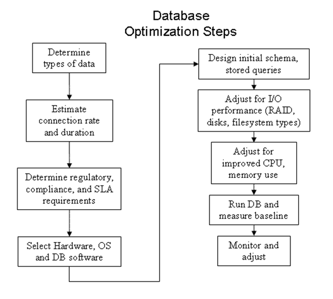
The first task is to make sure the database is running on appropriate hardware. Modern SCSI (such as SAS) may be best but SATA will work well too. Make sure it is modern or it may not support write barriers correctly. Use enterprise grade disks. Aside from spinning 2 or 3 times as fast as consumer grade ones, the firmware is better and more predictable (replacing a consumer grade disk, even with the same model, may not result in the same disk firmware.) Enterprise disks can also have non-volatile write caches (backed up with a battery or large capacitor).

Next, decide on central storage (SAN or NAS), or DAS. DAS may perform better (no network latency and no HBA, network switch, or OS write caches between your OS and the drives) but are not as flexible and may cost the same or more than central storage.

Turn off any OS LVM or software RAID. As for RAID, most database servers will work best with RAID 10. This give similar reliability to RAID-5 or RAID-6, but without parity calculations to slow down writes.

Finally, you will do best if you use the lower numbered cylinders (outer edge) of any spinning disks for the logs and database tables, and use the slower inner cylinders for OS and other system files. SSDs will work even better.

You need to monitor CPU usage (mpstat), RAM usage (free or vmstat), and disk I/O (iostat). (Linux tools; Unix may have different tools.) By monitoring these, you can see if a lack of hardware resources is the problem (and view trends over time, to predict when hardware upgrades might be useful).

Two key points for the SA are to use a safe filesystem type (e.g., ext4 or XFS, but not JFS or ReiserFS), and to force disks to write data immediately (known as direct write) by turning off any hardware disk buffering/caching (via hdparm -W 0), unless using a non-volatile buffer. Turn off any kernel buffering too! (Otherwise the DBMS thinks the data has been written when it may not have been; so crash recovery may lose/corrupt data.)

With ext4 filesystems, you can control the journaling feature: no journaling (write-through cache) with the mount option data=writeback, ordered writes (only filesystem metadata is journaled, but the by writing data then the metadata makes this fairly safe) with the mount option data=ordered, and journal (everything is journaled; safest but slowest) with the mount option data=journal. Best advice is to use journal mode and change to ordered mode only if performance is bad and changing this seems to make a difference.

Different types of filesystems work better with DBs than others. Using any FAT filesystem for a serious DB will cause poor performance. Using something like JFS or ext2 can improve performance at the cost of safety (not all writes are journaled). Using a journaling filesystem or RAID-1 (or similar) works best for DBs that don’t do that internally anyway (but most do, with a transaction log file). Note that without filesystem journaling, the transaction log file can become corrupted in a crash. Using tablespaces, you can put that log on one filesystem and the data on another.

Depending on how critical the data is, you may not want to use direct write as it slows down access to other files on that disk volume. With a decent UPS the small safety gain may not justify the performance loss. On the other hand an important DB shouldn’t share a storage volume with other files; it should have one or more storage volumes of its own. Also consider that with SAN/NAS/external RAID/JBOD storage systems, you may not have control over this, and in any case there are many caches between the server’s memory and the disk platter (the HBA, network switches, NAS head).

Creating a separate partition and filesystem just for the DB files works better than creating those files in (for example) the root file system with lots of non-DB files. Using separate filesystems for indexes, table data, and transaction logs can also greatly improve performance, especially if the different filesystems are on different disk spindles.

Either use a faster filesystem type and RAID-0 and let the DBMS handle those issues, or tune the DBMS to not bother with journaling (except for the logs) and/or mirroring.

Once the hardware is selected and your data is safe, then consider performance tuning. Poor performance will result when using a DB on a default filesystem type with default settings. A poorly tuned system can be much slower (10 times) than a properly tuned one! The different can be between minutes and days to execute some query. For example using Oracle on a FAT32 or ext4 filesystems with RAID-1 when Oracle uses different block and stripe sizes, journals writes to its files, and possibly mirrors the tablespaces, is not going to be fast!

First off, make sure you use a modern kernel version. Many have improved disk software a lot in recent years (2015). After choosing the file system type, set FS parameters.

Block (cluster) size can have a big impact on DBMS performance, particularly when running a database much bigger than system memory. One way to solve this problem is to reduce the value of the file system cluster size (maxcontig parameter) so that the disk I/O transfer size matches the DB block size. Another solution is to enable file system Direct I/O by mounting the file system with the right option (--forcedirectio for UFS), since file system Direct I/O will automatically disable the read-ahead. In addition, since MySQL has its own data and cache buffers, using Direct I/O can disable the file system buffer to save the CPU cycles from being spent on double buffering.

For most RDBMs the default OS value for disk read-ahead setting is too small, usually 256 (= 128 KiB on older drives). A good value should be 4096 to 16384. To set on Linux, use either hdparm or blockdev --setra (usually from rc.local). Next, mount the filesystem(s) with noatime. These two measures are probably the most important ones to improve performance.

The final OS tunable parameters to worry about are for OS caching and swapping. On Linux, set vm.swappiness to 0 (default: 60) to make the system avoid swapping as much as possible. (The trade-off is a smaller disk cache, but that’s worthwhile for most DBs.) To also help prevent swapping, set vm.overcommit_memory to 2 (never overcommit memory). Lastly you can control how many dirty memory pages the OS will allow to be outstanding before flushing them to disk; too many and the delay when the flush does occur will be noticeable, especially if you have lots of RAM. You can set vm.dirty_ratio to 2 and vm.dirty_background_ratio to 1 if you have more than 8 GiB of RAM. (All of these settings can be changed using sysctl, or directly using the /proc system. Make sure you set these at boot time, either by editing sysctl.conf or rc.local.)

One of the most important steps to tuning a DB is to create a good set of indexes. (This is likely more important than messing with tunable parameters.) Without proper indexes for you tables, many queries rely on sequential (linear) searching. Having too many indexes can also hurt performance, as the system must maintain all indexes whenever a table is updated. The primary key column(s) should be indexed (default for MySQL). Other columns may or may not benefit from indexing. By using the EXPLAIN command to show you details of the most common queries, you can determine which other indexes might help.

Bad performance can be the result of poor DB management: most DBMS use DB statistics (row counts, etc.) as input to the query optimizer. If these stats aren’t automatically updated by the DBMS and you don’t update them regularly, the optimizer can do a spectacularly poor job. For example, if the stats say a table with 100,000 rows has only 10 rows, then most optimizers would scan it sequentially because a sequential scan on a table that fits in one disk block will always be quicker than indexed access. You should turn on auto-stats (or whatever that feature is called on your DBMS) if that’s an option, or manually update them from time to time otherwise.

Performance also depends on the amount of writes versus reads for your application. Filesystems are typically designed have reads as fast as possible, and the difference in read and write speeds can be very noticeable.

If using NAS or SAN, network congestion is another factor.

Many enterprise-class DBMS (e.g., Oracle) don’t require a filesystem at all and can manage the raw disk space themselves. This feature is often referred to as “tablespaces”, each of which can be thought of as a file holding the DB data and meta-data. (With PostgreSQL, tablespaces sit atop regular filesystems.)

Setting the DB cache sizes is important as well, or the files used for the DB will end up swapped to disk and the frequent dirty page writes will slow down the whole system.

Keep in mind monitoring and backups: If using a filesystem the DB gets backed up (and disk space gets monitored) by your normal filesystem tools and procedures. If using raw disk volumes then you must use your DBMS system to monitor and backup the data using a separate procedure. Have an appropriate backup policy (SLA) and restore procedures. Often a monitor process must be kept running too, for security, compliance auditing, and baselining purposes.

The bottom line is for small or web site DBs that are mostly read-only, a filesystem based DB should be fine. For large OLTP systems, you need to have the DBA and the system administrator work together to tune the disk layout, the filesystem types used, and the DBMS itself. If using some enterprise DBMS such as Oracle that handles much of what the filesystem and RAID system can do itself, using a raw disk volume (and properly tuned DB) will result in the greatest performance for OLTP systems.

MySQL (and MariaDB) Specific Tuning

MySQL is a single-process, multithreaded application. The main thread is idle most of the time and “wakes up” every 300 milliseconds (msec) to check whether an action is required, such as flushing dirty blocks in the buffer pool. For each client request, an additional thread is created to process that client request and send back the result to each client once the result is ready.

MySQL includes several storage engines including MyISAM, ISAM, InnoDB, HEAP, MERGE, and Berkeley DB (BDB), but only InnoDB storage supports ACID transactions with commit, rollback, and crash recovery capabilities, and row-level locks with queries running as non-locking consistent reads by default.

InnoDB also has the feature known as referential integrity with foreign key constraints support, and it supports fast record lookups for queries using a primary key. Because of these and other powerful functions and features, InnoDB is often used in large, heavy-load production TP systems.

MyISAM (and ISAM) is for simpler applications (e.g., PHP blog, catalog data, and other non-OLTP applications). This has fewer features and limited scalability, but can provide superior performance (esp. connection speed) when you don’t need those features. You can use different engines for different tables in the same database, to get the maximum performance and safety.

MySQL has peak performance when the number of connections equals roughly 4 times the # of CPU cores. By estimating the number of concurrent connections, you can plan how large a SMP or cluster to use (i.e., how many DB servers are needed).

MySQL doesn’t access the disk directly; instead, it reads data into the internal buffer cache, reads/writes blocks, and flushes the changes back to the disk. If the server requests data available in the cache, the data can be processed right away. Otherwise, the operating system will request that the data be loaded from the disk.

Use EXPLAIN query to see what MySQL does. Use this insight to see where to change queries and/or add indexes. Tuning your queries and adding the required indexes is the best way to affect performance.

Once you’ve chosen the proper filesystem types, created the appropriate number of filesystems for your database, set their options and mount options correctly, and set the OS tunable parameters appropriately, it is time to consider adjusting the database's internal tunable parameters. Normally, that is left for a DBA to handle, not the system administrator (MySQL has over 430 tunable parameters!). But there are some performance measures you can consider for MySQL (and MariaDB):

· For applications where the number of user connections is not tunable (i.e., most of the time), the innodb_thread_concurrency parameter can be configured to set the maximum number of threads concurrently kept inside an InnoDB. (Other threads are kept waiting their turn.) If the value is too small under heavy load, threads will be kept waiting and thus performance will suffer. You need to increase this value when you see many queries waiting in the queue in show innodb status output. Setting this value at 1000 will disable the concurrency checking, so there will be as many threads concurrently running inside InnoDB as needed to handle the different tasks inside the server, but too many requests at once can also hurt performance.

· table_open_cache is the maximum number of simultaneous open files MySQL will request. Since each table is a separate file, you should set this to at least the number of tables used in your most complex query, times the number of DB connections you allow from clients. The default value (for MySQL 5.5) is 400 (used to be 64) and a real-word DB may have hundreds of tables, dozens at a time used in queries, with dozens to hundreds of open connections from clients. Note your OS must allow that many open files per process.

· The query_cache_size is the amount of memory to use to store the results of previous queries. This parameter can be set to 128MB or less, to provide better performance if usually many clients do read operations on the same queries. For some reason, this is set to zero on MySQL 5.6!

· The modern MySQL and MariaDB use the InnoDB back-end by default. The parameter innodb_buffer_pool_size determines how much memory the DBMS will request from the OS. On a DB server, you will get better performance from your system if you assign memory to this buffer pool, rather than a general OS page (disk) cache. The default value of 8 Mbytes is too small for most workloads. You will need to increase this number when you see that %b (percentage utilization of the disk) is above 60%, svc_t (response time) is above 35 msec in the iostat –xnt 5 trace output, and a high amount of reads appear in the FILE IO part of the show InnoDB status output. However, you should not set the cache size too large. If you do, you run the risk of expensive paging for the other processes running without enough RAM, and it will significantly degrade performance. For systems running a single dedicated MySQL process only, it should be fine to set this parameter up to a value between 70 and 80 percent of memory since the footprint of the MySQL process is only around 2 to 3 Mbytes.

· Another parameter to tune is key_buffer_size, which defaults to 1MB on older versions, and controls the size of the common cache used by all threads. With >256MB of RAM, set to 64M at least.

Scaling and Reliability

DBs are often a vital part of an enterprise, and must be highly available. This often means using some duplicate hardware in order to improve reliability (includes servers and disks). Duplicating the data on multiple servers is called replication. Also clusters are sometimes used to provide transparent failover and load balancing. In really large DBs (“big data”), tables are often split into shards. Such a distributed DB requires the query to figure out which shard holds the data requested, or to query each shard in turn and merge the results. (Example: DNS data is distributed and replicated.)

Most of these DB topics are beyond the scope of Sys Admin, certainly beyond the scope of this course. You are encouraged however to know these terms and concepts in a general sense.

Other Types of DataBases

Besides Relational databases, other types are used. One type is called a time-series database, used for storing event and metric data. Such databases are commonly used for monitoring systems (discussed in the vAdmin II course).

Blockchain is a new (2008) type of database, used for many purposes. A blockchain serves as the basis for some cryptocurrencies such as Bitcoin (the first public blockchain) and Ether. At its heart, a blockchain is a list of blocks of records. Every so often, a group of records is collected into a block which is added at the end of the list. Strong cryptographic methods are used making any changes to the blockchain very difficult. This means the blockchain can be used as a ledger that cannot be rewritten and can be verified by anyone with access. A typical blockchain block holds transation records (each digitally signed), plus a hash of the previous block, a time-stamp, and possibly other data. As of 2017, many companies are experimenting with blockchain technology to see if it can work better than traditional databases for particular applications.

Lecture 19 — Printing Concepts

An application creates a printjob, which is put into a spool directory (a.k.a. queue directory or print queue or just queue). A printer daemon (a.k.a. spooler) is a program the periodically examines the spool directory for any printjobs, tracks the status of printers, and sends printjobs to printers. (Spool is an acronym for System Peripheral Operation Off-Line, but I don’t believe this myself.)

In olden times this might’ve been as simple as cat printjob >/dev/lp0. KSR-33 TeleTYpe had uppercase letters only. Line Printers had 132 chains of letters and could print a line at a time. Later page at a time printers were developed. Laser printers came later, originally only publishers could afford these phototypesetter machines (CAT, Linotype). This meant that primitive word processors were very limited in their effects: bold (by printing twice), over-strike, and underline. Boring! Other old printer technologies include ASCII printers, daisy-wheel, and dot-matrix. (Such dumb printers can be quite useful to attach to a parallel port and send log info, which is just plain text, to the printer.) Controlling the printer’s available features meant using special printer codes embedded in the document to be printed (originally human typesetter instructions, such as “.sp”). (See the Typewriter Symphony Youtube video.)

Modern printers evolved from the dot-matrix printers, and include laser printers and ink-jet printers. The output quality of these printers is controlled by the dpi (Dots Per Inch, hxv, e.g., 600x600dpi). Such printers allow fancy looking output in various fonts, and not just text. Now word processors and other programs could use fancy printing, but the word processor document format is no longer just text and includes font and other embedded information (e.g., graphics). This document must be translated from some proprietary word processor format (e.g., MS Word) to the language the printer understands, the page description language or PDL.

Over time, two PDLs dominated the printer market: Adobe’s PostScript (Unix std PDL) and Hewlett-Packard’s Page Control Language or PCL (which evolved from printer escape codes). This translation is controlled by two bits of software. The printer driver knows the specifics of a given printer: paper size, dpi, features supported, and the communication details; that is, how the computer talks to the printer. The actual software that communications with printers is known as the backend. The other is the print filter, which knows how to translate one or more document formats into some PDL. (Analogy: Windows Add a printer means to install a print driver; MS Office ships with print drivers = print filters.) Note it is common (unfortunately) to use these terms interchangeably.

There are efforts to reduce the number of print filters needed, by standardizing the document format between applications and vendors. Some examples include PDF, MS OOXML, and ODF (Open Document Format used by OpenOffice and LibreOffice). PDF is the default PDL in CUPS 1.6 and newer; older print systems often used PostScript as the PDL.

As of 2014, all important desktop applications (GTK/GNOME, Qt/KDE, LibreOffice, OpenOffice.org, Firefox, Thunderbird, ...) send print jobs in PDF and not in PostScript any more, by default (at least on Linux systems).

Print filters can also perform accounting or even redirect print jobs across a network to a remote printer.

Most Unix systems include a suite of filters to translate various formats to PostScript, which has become the system standard format in Unix. So what if your printer is a PCL, GDI, or other type of printer?

Many generic (or dumb) printers without PostScript use ghostscript to translate Postscript to their PDL (or to strip the graphics and add printer codes in the text, for really old printers). GhostScript can translate PostScript to any of a few hundred different dumb printer formats.

The inventors of GhostScript, Artifex Software Inc., have now merged the commercial version with the free version (which had bug fixes and new features delayed by one year), and will provide better support for PDF documents, a format many printers can support natively.

Some non-PostScript printers include GDI (a.k.a. winprinter; GDI is the system standard graphic format for both screen and print) printers or PPA (from HP) printers. Such printers have no CPU, RAM, or rendering engine, so they’re cheaper. The work is done via software on the host: appl --> (PS-->) GDI --> (video driver or printer driver) --> bit-map. HP printers usually support both PCL and PostScript, and traditionally work well (especially for Unix).

Local and Remote Printing

Local printers (a.k.a. attached) attach to a port on the host. Usually parallel ports are used for printers. These ports are named /dev/lpn where n=0,1,2,... On Linux (/dev/lprn or /dev/parportn are sometimes used instead). (Serial ports can also be used. These are /dev/ttySn on Linux.) Modern Printers can attach to USB ports, /dev/usb/lpn on Linux.

Remote printers are printers locally attached to some remote host that runs a print server. Besides the normal printing issues you must have the client and server communicate using some protocol: LPD (RFC-1179), IPP (Internet Printing Protocol), CIFS (SMB), and even HTTP are common. If using a modern printing API, applications can directly send print jobs to queues on remote hosts.

If your applications use an older print API the local host must run some minimal print server (queue software). The administrator defines local queues that (behind the scenes) forward print jobs to remote print servers. Local applications thus only need to use what they think is a local printer. However this means a more complex setup on every host, and if a printer is upgraded or moved to a different host (or a print server changes its IP address), every host will need updating!

Network printers may have their own spooling software (commonly using the JetDirect print server, a tiny special purpose host that only runs a print service) or they may be dumb and rely on some host to provide spooling. In this case the administrator must make sure there is only one host controlling the printer and no host sends print jobs directly to that printer.

Use Samba to connect to a remote Windows print server for printing via CIFS/SMB. (The name for one popular, old version of SMB is CIFS. Even though SMB2 and SMB3 are very different than SMB1/CIFS, the name “CIFS” somehow stuck. Try to avoid using it.) You can setup a Samba server to allow remote Windows clients to use your local printers (must configure /etc/smb.conf to allow Windows clients to see your printer in their network neighborhood). Note that Windows servers can be configured to use the LPD protocol.

(Samba can also be configured to provide print services to Windows clients.)

Usually there is one print queue for every printer, local or remote. However it is possible to define multiple printers for the same queue (HCC did this in the open lab when we used slow printers), and multiple queues for the same printer (usually each queue has a separate priority or requires paper changing). A printer destination is the name of a queue (which is normally the same as the printer name). Note printer destination names may be restricted to 14 alphanumeric, case-insensitive characters.

Common Print Systems

LP Print System - derived from the original AT&T system, LP doesn’t support remote printers. All modern systems have grafted on some other system to support this. (Used on Solaris pre-11, HPUX.) nsswitch.conf can be used to tell the local system where printers configuration information is (files, LDAP, NIS, etc.).

LPR Print System LPR derived from the BSD print system, and is still widely supported on Unix, Linux, and even Windows NT. See RFC-1179 (a.k.a. the LPD protocol). Access control is provided by two means. First, all requests must come from one of the machines listed in the file /etc/hosts.equiv or /etc/hosts.lpd. Second, if the rs capability is specified in the /etc/printcap entry for the printer being accessed, lpr requests will only be honored for those users with accounts on the machine with the printer.

LPRng Print System LPRng is a re-worked LPR from the ground up, with new configuration and access control files: /etc/lpd.conf (LPRng configuration file), /etc/lpd.perms (LPRng printer permissions), /var/spool/-printer* or .../lpd/* (spool directories and printer-specific printcap info).

CUPS Print system Common Unix Printing System (yes I know it’s redundant). (See www.cups.org.) Used on Linux, Solaris 11, and many other OSes. CUPS uses the Internet Printing Protocol (“IPP”) as the basis for managing print jobs and queues. The Line Printer Daemon (“LPD”), Server Message Block (“SMB”, renamed “CIFS” (Common Internet File System) and then renamed in later versions back to “SMB”; the name “CIFS” somehow lingers on), and AppSocket (a.k.a. JetDirect) protocols are also supported with reduced functionality. CUPS adds network printer browsing and PostScript Printer Description (“PPD”) based printing options to support real-world printing under UNIX. (Note CUPS includes print filters for text, PS, PDF, and other std formats.) Some decent (but perhaps outdated) articles can be found at openprinting.org - V.CUPS-Filtering-Architecture and LinuxFoundation.org - openprinting group home.

When printing to a Windows printer, you often need to specify NetBIOS share names. A common error is to forget backslashes have special meaning to the shell. Use forward slashes instead, or doubled back slashes.

Print Filter Collections

APSfilter is a filter collection for LPR or LPRng systems, which can auto-detect input file formats and translate PostScript, ASCII, TeX DVI, PCL, GIF, TIFF, HTML, PDF, and a number of bitmapped graphic formats to PostScript. It then uses GhostScript to support non PS printers. APSfilter utilities setup the LPR printcap file and create the print queue directories, including configuration data and correct permissions. Magicfilter is similar.

Foomatic is a print filter system designed to support any spooling system (including CUPS). It is a part of OpenPrinting’s print filter database environment Foomatic and is a standard part of all modern Linux distros.

You can find filters that ship with CUPS in /usr/lib/cups/filter/.

The main filter/RIP (Raster Image Processor) wrapper foomatic-rip works like APSfilter to detect input format and convert to PostScript. It then uses a collection of PPDs and printer drivers to make the final translation for the actual printer driver (note GhostScript may be used as the printer driver). See www.linuxfoundation.org/.../foomatic.

PPDs are text files that describe all printer options and features. Originally, PPDs were designed by Adobe just for PostScript printers (the name means PostScript Printer Description). CUPS extended their use to all printers. Find PPDs at openprinting.org/printer_list.cgi. Most (if not all) print filter collections include an extensive collection of PPDs as well. The definition of the PPD file syntax can be found at partners.adobe.com.

Most Linux printer drivers use foomatic-rip which is a standard part of all modern Linux distros. Foomatic-rip is also used with Solaris.

You can find PPD files (and some CUPS filters) in /usr/share/ppd/. Foomatic PPDs are in /usr/share/foomatic/db/source/PPD/.

User CLI Utilities and Configuration

Users can have ~/.printcap (LPD) or ~/.printers (Solaris) files to support their own printers. CUPS users can have ~/.lpoptions to override per-system (or per server) settings.

The lpr and lp commands take cmd line args to determine what printer destination to use, what print filter to user, etc. (Solaris: see ppdmgr(1M).) These CLI utilities came from the BSD and AT&T print systems respectively, but today all print systems provide both commands (perhaps one with limited functionality. Many simple GUI applications simply invoke one or the other to print. (Most modern applications use some printing API).

There are defaults for everything: The system check for PRINTER and LPDEST environment variables if no cmd line args are present, and .printcap/.printers if present or a system-wide default printer, which is a printer named lp or the first printed defined in printcap/printer.conf if no lp printer. lpoptions can be used to override system defaults (CUPS).

With CUPS, use lpstat to see printer and queue information: lpstat -dap. To set a default queue (destination, or printer), use: lpoptions -d name. To see your current printer settings (in ~/.lpoptions), use: lpoptions -l. (Note that when run as root, lpoptions changes the system-wide defaults in /etc/cups/lpoptions, not the root user’s settings.)

Use pr to print text files with page headers.

Use col -bx to strip (some) control characters, e.g., printing man pages.

Some print filters can be invoked directly with the results piped into lpr. Use a2ps, enscript, or mpage for 2-up printing and other effects such as controlling margins for plain text. (ex: mpage -m38lt.) You can edit the print filter wrapper (shell) scripts used with some print systems. Edit /var/spool/lpd/lp/mf.cfg to invoke mpage with various arguments with LPRng.

enscript is a popular print filter. It can convert a text file to PostScript, Rich Text Format (RTF), and HTML. You have many, many options to control what is printed and how. For example, you can convert a text file to a two column PostScript file using landscape mode, with the command: enscript -2 -r -p psfile.ps file.txt. Or print Bash shell scripts with syntax highlighting as HTML, with: enscript -Ebash -p - -w html script.sh.

Printing Related Commands

Description	AT&T (lp)	BSD (lpr) LPRng	Solaris pre-11	CUPS
Print facility config	lpadmin	lpc	lpset, lpadmin, lpsystem	lpadmin, GUI, lpoptions
Submit a print job	lp	lpr	lpr/lp	lpr/lp
Printer daemon	lpsched, lpshut	lpd	lpsched, lpshut	cupsd
Enable a printer	enable^†	lpc	lpset/lpc, enable	cupsenable
Disable a printer	disable	lpc	lpset/lpc, disable	cupsdisable
Enable a print queue	accept	lpc	lpset/lpc, accept	cupsaccept
Disable a print queue	reject	lpc	lpset/lpc, reject	cupsreject
Cancel a pending print job	cancel	lprm	cancel	cancel/lprm
view printing status	lpstat	lpq	lpstat	lpstat, lpinfo, lpq, lpoptions
Printer database (in /etc)	printcap	printcap	printers.conf	cups/*
Access controls (in /etc)		lpd.perms, lpd.config (hosts.lpd)	lp/printers/name/*	cups/cupsd.conf (use lpadmin)
Spool directories (in /var/spool)	lpd/*	print/* or lpd/*	lp/*	cups/*

^† Note: Bash uses enable as an internal command. You should use the complete pathname to the enable command every time, to avoid conflicts.

Configuration

Use LPRng command checkpc (check print configuration) command.

GUI tools for printer setup: RH printconf, Sun Solaris Print Manager

Red Hat’s GUI printer config tool rewrites /etc/printcap each time, so changes made manually are lost. Put your changes in /etc/printcap.local instead.

To configure CUPS, edit files under /etc/cups/, run lpadmin or other CLI tools, or use the GUI by opening the URL of http://localhost:631/ in a web browser.

CUPS restricts who can admin the CUPS system and even who can use it to print. The default on Fedora is to allow any user in one of these groups (setting in cups-files.conf):

SystemGroup sys root wheel

So when using the GUI, either supply the root user and password, or your own username and password if you are a member of group wheel.

To switch print systems, reset symlinks in /etc/alternatives via the RH and Debian alternatives command.

A common problem with text printing is Stair-stepping. This can be fixed by enabling LF -->CR/LF in the print filter configuration used for text files.

CUPS on Fedora have known issues with the default configuration! Why this has never been fixed, I have no idea. But if you find you cannot use CUPS, try setting SE Linux to Permissive at boot time (edit the file /etc/selinux/config), and rebooting. (The alternative to disabling SE Linux is to trouble-shoot the issues and fix the policy yourself. Start by running “restorecon -Rv /”, then reboot and fix the policy errors one at a time until there are none left. You may find you also need to enable a boolean for CUPS (“setsebool -P cups_execmem 1”).)

By default, CUPS on Fedora sends error messages to the journald daemon and not /var/log/cups/error-log; you then read CUPS related log messages with “journalctl -b -u cups”. It is possible to configure CUPS to send logs to files instead. If you do that, also enable log rotation for those files.

Windows username to use at HCC-DM: PRTUSER, pw=PRTUSER

CUPS info: Use “smb://user:password@domain/server/share” as a URI to connect to a Windows printer, e.g.:

smb://PRTUSER:PRTUSER@DM_ACADEMIC/DM_TECH_B/Tech_461

xojpanel: a GUI app that displays an HP printer’s LCD panel on your desktop.

Linux uses /etc/papersize to tell utilities the preferred size: letter, legal, a4, etc. (This can be over-ridden with some env. vars: PAPERSIZE, LC_PAPER, or PAPERCONF (points to a different file to use). See papersize(5) for more, also paperconf(1) and paperconfig(8).

Discuss firewall, SELinux issues (turn off initially to print).

Solaris pre-11CLI Printer Setup

[From: www.sun.com/bigadmin/content/submitted/duplex_printing.html]

You can use lpadmin to set up a print queue. The exact options differ from Solaris printing and CUPS; see also lpoptions, lpinfo, lpstat, cupsenable, and accept. Here is a Solaris example for the Brother HL-5170DN, which is attached to the network with the host name laser:

# lpadmin -p myprinter -v \
/dev/null -m netstandard_foomatic -o protocol=bsd,dest=laser \
-T PS -I postscript -n /usr/local/ppds/br_5170_2.ppd

In the above, -T PS and -I postscript indicate that this is a PostScript-capable printer; you need this to prevent the printing subsystem from trying to send ASCII banner pages to it. The -n option indicates the location of the PPD file. You should use the real location of your file, which might be a file in /usr/lib64/lp/model/ppd, or it may be somewhere else on the system. The -m, -v, and -o options basically configure access to the printer itself. If your printer is locally attached you might use this instead:

# lpadmin -p myprinter -T PS -I postcript -v /dev/ecpp0 \
-m standard_foomatic -n /usr/local/ppds/br_5170_2.ppd

You also need to configure lpsched to enable both the queue and printer. Use these commands:

# accept myprinter
# enable myprinter # if using bash, use a pathname!

You can now print duplex pages using one of the following command syntax:

% lp -d myprinter -o sides=two-sided-long-edge somefile.ps
% lp -d myprinter -o sides=two-sided-short-edge somefile.ps
% lp -d myprinter -o sides=one-sided somefile.ps

Setting Default Queue Options

To avoid specifying options every time, you set default options for a queue with:

% lpadmin -p myprinter -o sides=two-sided-long-edge \
-o banner=never

If your printer is networked, you can set up different queues with different default options. With CUPS, see the other lp* commands for available options.

Print Quotas and Accounting

CUPS supports page and size-based quotas for each printer. The quotas are tracked individually for each user, but a single set of limits applies to all users for a particular printer. For example, you can limit every user to 5 pages per day on an expensive printer, but you cannot limit every user except wpollock.

With CUPS, every printed page is logged in /var/log/cups/page_log, so one can read this file and determine who printed how many pages. These functions depend on CUPS filters reading the PostScript produced to determine page counts. Page logging is only available for drivers that provide page accounting information, typically all PostScript and CUPS raster devices. Raw queues and queues using third-party solutions such as Foomatic generally do not have useful page accounting information available. In addition, clients that render the print job internally without using CUPS filters can’t be accounted for.

If there is a problem when printing (e.g., a paper jam) after the CUPS filter has processed the job, the accounting will show the job as printed even though it wasn’t.

To restrict the number of pages (or Kbytes) which a user is allowed to print in a certain time frame, use the lpadmin command for the print queues:

lpadmin -p printer1 -o job-quota-period=604800 \
-o job-k-limit=1024

lpadmin -p printer2 -o job-quota-period=604800 \
-o job-page-limit=100

The first command means that within the “job-quota-period” (time always given in seconds, in this example we have one week) users can only print a maximum of 1024 Kbytes (= 1 MByte) of data on the printer “printer1”. The second command restricts printing on “printer2” to 100 pages per week. One can also give both restrictions to one queue. Then both limits apply.

While there is no way to query the current quota state for a particular user, any application can request a list of jobs for a user and printer that can be used to easily determine that information.

For more sophisticated accounting use (third party) add-on software which is specialized for that job. Such software can limit printing per-user, can create bills for the users, use hardware page counting methods of laser printers, and even estimate the actual amount of toner or ink needed for a page sent to the printer by counting the pixels.

A well-known and free software package for print accounting and quotas is PyKota: www.pykota.com

A simple system based on reading out the hardware counter of network printers via SNMP is accsnmp:

fritz.potsdam.edu/projects/cupsapps/

Current Problems with Printing

Printing is too complicated today! Every *nix variant requires its own printer drivers/filters, due to minor differences between distros. Also most cheap printers don’t directly support the standard (intermediate) print file format of PostScript.

One problem with having so many print systems available is that applications must be written to use a specific one or suffer limited functionality (if they use lp or lpr when CUPS API is available) or not print at all (if they use CUPS API when that isn’t the print system installed). It is hoped that CUPS will become universal but that hasn’t happened yet. (Many organizations have used lpshed, Solaris printing, LPD, etc., for years, and see no great incentive to change everything around).

With CUPS, printer features aren’t discovered but listed in a PPD. Printer feature discovery would be much better (as even a printed that can staple may be out of staples now). Another nice feature missing currently is to save frequently requested options as a job ticket, so you can easily set up a print job. Also there is no standard way to easily print from PDAs, cell phones, BlackBerries, etc., using (say) Bluetooth or USB.

The Future of Unix/Linux Printing

[From www.onlamp.com/pub/a/onlamp/2007/09/20/printing-trends-in-linux.html]

The Open Printing Working Group (OLPW), the Linux printing group formally under the control of the Free Standards Group is now (like the LSB) under the Linux Foundation (linux-foundation.org) umbrella. The OLPW works closely with the Open Print Working Group (OPWG) of the IEEE Industry Standard and Technology Organization (ISTO) so their work should apply to Unix and Linux systems. This new open printing standard is called the Open Standard Print API (or PAPI).

Instead of applications having to support many different print systems, the application-neutral, print system-neutral middleware PAPI can be used. This API is the same regardless of which print system is used.

It is easy to configure PAPI for different print systems and the applications won’t know the difference. PAPI has interfaces for LPRng, CUPS, etc. Currently an open source version of PAPI is available from sourceforge.net.

The OPWG is backed by most printer vendors who want to provide printing support for Linux (and Unix) and realize they can’t afford to put in the same effort dealing with each distribution that they put into dealing with Microsoft. About half of the OPWG’s volunteers work for printer vendors or ISVs. See OpenPrinting.org for more information.

These groups are also working on standards to support automatic printer driver installation (similar to the Windows printer installation system). However security is a concern for this; no doubt the drivers will be required to have digital signatures and other protections before automatic driver download and installation becomes useful.

Printer feature discovery is increasingly available by using printers that support SNMP. This support can be incorporated into CUPS, allowing easy and accurate printer dialogs, and better printer management.

The new LSB version (3.2) will cover printing standards, so OS neutral print drivers/filters will soon be used. LSB has standardized on CUPS and Foomatic.

One of the decisions already made and slowing being accepted is to switch the standard Unix print job format from PostScript to PDF. This format has many important advantages: PDF is the common platform-independent web format for printable documents, Portable, Easy post-processing (N-up, booklets, scaling, ...), Easy Color management support, Easy High color depth support (> 8bit/channel), Easy Transparency support, Smaller files, Linux workflow gets closer to Mac OS X, for some printers may save the CUPS-required GhostScript processing step.

(The switchover to PDF as standard Unix print job format is work in progress.)

One of OPWG’s newest subprojects is working on ways to quickly test whether a printer driver is present and supports all of the printer’s features and whether the complete print workflow chain of software is present and installed. This should ease management and installation issues.

Support for PDA and other small devices appears some way off at present. Although neither a spooler nor GhostScript are needed, a small printing stack of software that has a GUI for printer discovery, feature discovery, printer (and feature) selection, etc.

Lecture 20 — Adding and Managing Users and Groups (User/account management)

Have a policy and procedure for creating new users and groups. Questions to ask:

· Who gets accounts on which machines? Who decides this? Who is actually authorized to create the accounts?

· Are accounts local to a system/location, or global (to the organization)?

· Are all accounts centrally managed, or can local SAs administer local accounts (and with what policies)?

· Are the policies and procedures different for local vs. global accounts?

· What is the procedure to request a new account (or disable or remove an account)?

· When do accounts expire?

· How are account names chosen (the naming policy)?

· What is the password policy (who can change them, when do they expire, what is the required strength)?

· How many accounts may a single user request at one time? (Ans: one)

· May accounts be shared? (Ans: no)

· How much disk space does a user get? What happens if they exceed their quotas?

· What email access is available (web mail, IMAP, POP, SMTP, ...)?

· What printer access is provided (how many pages, to which printers, and at which time of the day)?

· From which workstation(s) may the account be used?

· Is remote access provided for this user?

· Is accounting to be used for this user? If so, how much capacity can be used and for what?

· Employers and employees should be sure to establish, in writing, whether a social media account (Facebook, LinkedIn, Twitter, etc.) is a personal account, or belongs to the employer. This matters if you use your account for any business purposes, including just listing your current employer and job title. (One PA woman had the employer take over her LinkedIn account, replacing her information with that of her successor at the company. The courts ruled in the company’s favor.)

· What additional access does the user require? (To which additional groups should the user be added?) Note additional access may require additional configuration: database access, administration access, physical access to machines, Kerberos (Samba) access, NFS access, email access, protected website access, FTP access, crontab/at access, remote (dialup/VPN) access, Internet access, other server access, etc.

Case Study: User policy at kernel.org

Kernel.org currently supports ~300 users (those with logins), who are usually either kernel module maintainers or high-profile developers. To qualify for a kernel.org account, people have to either be listed in MAINTAINERS or receive a special approval from the steering committee (Linus, Greg KH, H.P.Anvin, Ted Ts’o).

We also require that people are in the kernel.org PGP web of trust, which means that before anyone is given access, they must have PGP signatures from at least 3 other kernel developers who already have a kernel.org account.

Creating accounts

Point out that many user/group accounts created for special purposes: ftp for anonymous ftp user, nobody for apache user, etc. (Usually one account per service). These are called system accounts. Never add additional users to system groups!

Some UIDs (and GIDs) have special meanings: 0 means root access; other special privileges may be granted for for UIDs (and GIDs) less than 10, 100, 500, or 1,000, depending on the system. These IDs are for the system accounts.

On most systems, especially when single sign-on is used, you should make sure your UIDs and GIDs follow the modern *nix standard:

UID/GID 0 is reserved for root.

UIDs/GIDs ranging from 1-99 are reserved for other predefined accounts, such as “3” from “adm” on Linux. Red Hat (including Fedora) includes a list of predefined system UIDs and GIDs, in the file /usr/share/doc/setup/uidgid.

UIDs/GIDs ranging from 100-999 are reserved for other system accounts, such as for a web server (RHEL <7 reserves only up to 499).

Normal users have UIDs/GIDs of 1,000 or greater (on RHEL <7, they start at 500).

Setup these so no logins (or FTP) is allowed for such users: discuss /etc/shells (valid shells), /bin/false, and no shell at all. Also disable account in shadow (no valid password, something like “!!no login” in the password field). (Solaris: *LK*.) Locked or invalid shell prevents ftp, possibly other services.

The systemd-sysusers command uses the files from the /etc/sysusers.d/ directory to create system users and groups and to add users to groups, at package installation or boot time.

Networks of computers (and even single hosts) can use a shared user account database: NIS, NIS+, Kerberos (Win2k and newer users this), LDAP, or others. Each user gets a single record in the database and can be authenticated on any machine in the network. (Example: YborStudent, DMSun, Windows network, all use a single DB so you have a single password for any computer at HCC.) These are known as global accounts. Each host may also have local accounts. (Where to find accounts is determined by PAM or nsswitch.conf or both.)

Accounts should always be created disabled initially. You should have and follow a password policy (strength, expires, ...), have a default shell, set a default web page to the company policies and procedures webpage (new user page which you create & maintain), decide which services to allow (telnet, website, printing, Internet access, NNTP (netnews) access, remote access, administration access, FTP, SSH, DB, chfn, crontab/at, Samba, ...), and configure such services as needed. /etc/default/* contains defaults for several programs including useradd. Don’t forget to set a default printer, any needed quotas (see below), NFS, and an initial password (use a password generation program such as pwgen or apg).

Use a custom script to add, disable, and remove accounts: samba.conf, htaccess, ... Your script can invoke useradd. Then it can add the user to DB access files and various groups, to setup accounting, quotas, website, email aliases, etc. Can also email user a “welcome” message, set first time home page for web browsers to new user info, etc. This way you don’t have to remember all the services and how to configure each. Just maintain the scripts.

Have policy for usernames. Don’t have long names. Don’t use periods (or other special symbols) in usernames (periods will mess up LDAP, NIS directories). While usernames are case-sensitive, email addresses are not. So it would be a mistake to have two user accounts “hymie” and “Hymie”. Use only 8 lowercase letters, digits, and underscores, and your names will work on all systems; a good idea if single-signon is used (or a possibility). For example, flast (‘f’=first name initial, ‘last’=up to seven letters of last name. Consider non-English names too; in some cultures, one name is the norm.)

A good policy is dept###, as in “it012” for the IT dept, using all lowercase letters and digits only. However, this makes it hard for SAs to match real names with account names. A common policy is to form usernames from the users’ names. This can cause problems when you hire the second “J. Smith” and you wind up with accounts such as jsmith2. There is also a security implication: if a cracker knows an employee’s name, they can easily guess the login account name. For greatest security, each account should have an email alias as well (again, to hide the real account names). In most environments, such security measures are not needed.

Usernames > 8 characters or that contain weird characters can crash some programs on Solaris, and cause security problems on any *nix system. In particular, the common practice of using periods in names is bad (can confuse chown and other commands).

Password policy: The file /etc/login.defs (Solaris equivalent: /etc/default/login) is the configuration file for the Shadow password Suite. /etc/login.defs contains settings from what the prompts will look like to what the default expiration will be when a user changes his password. The /etc/login.defs file is quite well documented just by the comments that are contained within it.

The login.defs file has a setting for minimum password length, but this setting is only used if the shadow suite is used, not for NIS or LDAP. Also passwd uses PAM to reject passwords, so configure that to set policy (discussed in CTS-2322). Both login.defs and PAM are checked when changing passwords.

Warning! Some (but not all) Linux security utilities use a common library for updating passwords, groups, etc., called libuser. The /etc/libuser.conf imports values from login.defs and /etc/default/useradd, and can over-ride those settings. Note useradd doesn’t use libuser.so while passwd does. When changing password policies, be sure to update all the policy files! Otherwise some commands will use different policies. (Yes there should be one password policy file, but nobody asked me.)

Password aging policies need to be defined as well. Besides the account expiration date, you can set a max password age (in days) after which the user will be forced to change it (at next login). You can also set a warning period. The poorly named inactive days is the number of days after which an expired password is no longer accepted (so the user is locked out).

Groups

A group is a collection of users who can share files and other system resources (i.e., a group of users with identical access needs). For example, the set of users working on the same project could be formed into a group. Each group must have a name, a group identification (GID) number, and a list of user names that belong to the group. A GID identifies the group internally to the system. Some GIDs have special meanings to the system (e.g., GID of zero.) The standard DB for group information is /etc/group.

(See web resources for group strategies).

The two types of groups that a user can belong to are the primary group, which specifies a group that the operating system assigns to files created by the user, and secondary (or supplemental) groups, which specify one or more groups to which a user also belongs.

Each user must belong to one primary group. Users can belong to up to 16 secondary groups (legacy limitation from RPC/NFS). If not using RPC/NFS a user can belong to up to 32 secondary groups (no limit on Linux kernel, on other systems max value NGROUPS can be configured).

Ownership of newly created files reflects the primary group, not any secondary groups. (A user can change the group of a file to any secondary group using chgrp.) A user can also temporarily change the primary group with newgrp (which starts a new shell), or permanently by updated the user database e.g., /etc/passwd.

To add a group without logging out and then logging back in (the normal way to have the changes picked up), you can try this hack:

exec su -l $USER

But this only works for the current shell (not all sessions at once), and will log you off if you mess up your password. Still, that’s not a big deal. The exec works with newgrp as well.

Some groups have special uses. On Solaris a user has to be a member of the sysadmin group (group 14) to use the Admintool software, but it doesn’t matter if group 14 is their current primary group. (Linux, BSD: wheel group may be used similarly.) With systemd, the log data for any user can be view if you are a member of the adm group. Many other groups are used as the group ID for particular daemons, or have other purposes.

Two other groups worth knowing about: members of group vboxsf (and root) are the only ones with access to VirtualBox shared folders; members of group wireshark (and root) can capture packets.

groups lists groups that a user belongs to, as will the id command. (To find out all groups for some user, grep for that user in /etc/group and in /etc/passwd (for primary group number; grep for that in /etc/group to get name).

When adding a user account, you must assign a primary group for a user or accept the default: staff (group 10) on Solaris. The RH default is to create a new group for each user. (This default can be changed.) The primary group should already exist (if it doesn’t exist, specify the group by a GID number). User names are not added to primary groups. (If they were, the list might become too long.) Before you can assign users to a new secondary group, you must create the group and assign it a GID number. Add/remove users to/from groups with gpasswd (Linux) or smgroup modify -m grp user (Solaris).

Account and Group Management Commands

GUI tools: redhat-*, system-*, admintool (and SMC) for Solaris, webmin (all systems).

Cmd-line: user{add,mod,del} (Linux note: using -p 'foo' sets the password field in shadow literally to foo, not to an encrypted version of it!) Discuss the -G option to set supplemental groups for users; use -Ga to append.

If using some single sign-on centeral user account database, these commands may not work correctly, as they generally only add users to system-local files (such as /etc/passwd). Other commands add/modify/delete users from LDAP or Active Directory (Kerberos) user databases.

group{add,mod,del}, gpasswd (Solaris: smgroup) (discussed below), passwd (Solaris version does more than the Linux version),

vipw, vigr, pwck, grpck, chage. (Also chfn, chsh; on Solaris use passwd.) Another (sometimes useful) command: last shows the last time a user has logged in.

Manually: edit the files /etc/{passwd,shadow,group,gshadow,skel,login.defs,libuser.conf}. Also configure PAM for login and password configuration.

Some systems may include commands for adding users in batches, or changing passwords in batches. For example, see the Linux commands newusers and chpasswd.

Set up quotas (discussed later) with setquota, edquota.

Warning! The standard commands to lock accounts (“lock-out users”) are passwd -l and usermod -L. However, these commands don’t lock the account!

What these commands do, is prepend “!” or “!!” to the password in /etc/shadow. (Solaris replaces the password with “*LK*” instead.) The idea is that any attempt to log in can’t succeed since nothing you enter can match such a password. However, this won’t prevent users from loggin in using SSH keys, or (on most systems), from running crontab or at jobs, or receiving email (which can cause programs to run via ~/.forward or ~/.procmail).

It works better to use some PAM modules to lock accounts, say pam_listfile.so to check a list of locked usernames, or pam_shells.so to check for a valid shell in /etc/passwd. Then you can lock accounts by adding the username to the list checked, or by changing their shell field to something such as /bin/false.

The standard way to lock out users is to expire their user account. If using the shadow suite, you can use “usermod -e 1” for that.

Systemd attempts to manage user processes and sessions. The systemd command to manage user sessions is loginctl.

Since version 230, systemd by default will kill all a user’s processes still running once the user logs out, including those started by nohup! It is possible to disable this “feature”. To do this, a system administrator can set the “KillUserProcesses=no” option in systemd’s configuration file /etc/systemd/logind.conf.

If just a few users needs to run processes that should be left alone by systemd, they must enable “lingering” for their account with “loginctl enable-linger username”, and remember to run commands with the systemd-run command preceding the nohup command (also the tmux and screen commands).

Setting up disk quotas on Linux — the short version

quotaon -pa # shows no quotas on

vi /etc/fstab # add usrquota and/or grpquota to options

mount -o remount /home # picks up new options

quotacheck -cMuv /home # create, initialize the quota DB

chmod a+r /home/aquota.user #permit users to check quotas
restorecon /home/aquota* #Update SELinux labels if needed

quotaon -a # start enforcing quotas

setquota auser soft-bk hard-bk soft-files hard-files /home

setquota -ta 604800 604800 # 7*24*60*60= 1 week grace

repquota -a

Disk Quotas

A disk quota is a limit on the amount of disk blocks and/or inodes a given user (or group) is allowed to use, per filesystem. Not all filesystem types support quotas; for those that do special mount options must be used to have the kernel enforce the limits. A special command toggles quote enforcement (quotaon).

When quotas are enforced (“turned on”) the kernel will track how many disk blocks and inodes a user is using, and update the quota database file(s). When quotas are not enforced, or the filesystem is mounted without the proper mount options, the databases do not get updated. Even when enforced, if a filesystem remains mounted long enough it is possible for the database to become corrupted. Periodically (and also typically at each boot) the quota database file(s) for each filesystem with quotas gets rebuilt using the command quotacheck. This command is also used to create the DB the first time you set up quotas.

If a user exceeds the quota limit for the number of blocks and/or inodes, the user won’t be able to allocate any more blocks/inodes but can still unallocate them (i.e. remove files). The system uses both a hard quota limit that can never be exceeded (while quota enforcement is on), and a lower soft limit that can be temporarily exceeded.

Once a user goes over the soft limit a configurable (per filesystem, not per user) grace period timer starts a countdown. As long as there is still some grace time left the user can still allocate more blocks/inodes. But once the grace period has expired (it will report “none” left) no further allocations are allowed. In addition the SA can configure the quotawarn system (run either by cron, manually, or by a login script). This will generate email and/or console warnings to the user if they are exceeding their soft quota.

Once the user has reduced their disk use to be under the soft quota limit, the grace period gets reset.

Some weird things can happen when you exceed your quota and your grace period has expired. If you have exceeded your block quota but not your inode quota on /home, you can still create files but they will all be zero length. This can prevent GUI logins, since X attempts to create ~/.Xauthority. (If the file can’t be created X will try to create it in /tmp instead). The file gets created but of zero length, and when X tries to use it the session fails. Depending on your login scripts even console logins may fail.

Commands: quota [-sugvq] to report on quotas. This is the one command regular users can use to see their own quotas.

quotaon [-a], quotaoff is used to turn enforcement on/off, per filesystem. (“-a” means turns on/off quotas for any filesystems listed in fstab with the mount options quota or usrquota or grpquota, or some such option; this depends on the options supported by that type of filesystem. See the mount command man page.) Running quotastats shows the kernel’s quota activity.

repquota will produce aquota report on Linux; the Unix command is quot. Running (as root) quotasync first makes the report accurate.

Use quotacheck [-anMguvR] to create or recreate the quota database file(s) on each filesystem (aquota.{user,group} in the fileystem’s root directory). The common (Linux) options include: -a = all FSs listed in fstab, -n=ignore duplicate entries (i.e., fix DB corruption), -M=don’t quit if can’t remount partition as ro (useful for root partition), -g=do group quotas, -u=do user quotas, -v=show even if =zero, -R=don’t do quotacheck for root. Typical use:

quotacheck -aRnguv; quotacheck -Mnguv /

Since the root filesystem cannot be mounted read-only while the system is running, we need to do a force quota check on the system which might result in inaccurate figures and can cause corruption to the quota files. For this reason, only check the root filesystem while the system is quiescent (e.g., in single-user mode, with no daemons running). It is advisable to have a partition plan where quotas on the root filesystem aren’t needed.

Easier is to pass the systemd option “quotacheck.mode=force” to the kernel from your boot loader. While not documented in systemd, creating a file named “/forcequotacheck” also works (thru F27 at least) to make the next boot check quotas.

Note that most filesystems treat the quota databases specially, and do not journal updates. As a result, it is usually required to rerun quotacheck after a crash. For Linux ext3 and ext4, there are special mount options to force quota updates to be journaled as well. (See mount(8) for the ext4 options of usrjquota and grpjquota.) A typical use would be:

usrjquota=aquota.user,jqfmt=vfsv0

Note two (rather lengthy) options are required to enable journaled quotas.

edquota : puts SA into vi to edit quotas: -g=edit group quotas, -t=edit soft limits instead of hard limits. I prefer to use the setquota commad line tool which can be scripted, or any GUI tool such as webmin.

warnquota can be used from /etc/profile login script or cron.daily. It needs to be configured with the fileystems to watch and the messages to show.

To turn on quotas use some simple GUI tool, or do these steps:

(1) Edit fstab and add usrquota,grpquota to options. (If not using group quotas, there is no need to enable and enforce them. Note some system use (or allow) quota in place of usrquota.)

(2) Create empty quota files in the root directory of each filesystem, e.g.
touch /home/aquota.{user,group}
(This is because the quotacheck command can edit these files but not create them, on some systems.) Verify the quota database files have been created with the correct permissions: chmod 644 aquota.{user,group} (If not readable, users can’t check their quotas, only root can!)

(3) Remount disk partitions to enable the new options:
mount -o remount,usrquota /dev/sda? or /dev/mapper/*
(If this fails, it maybe due to GVFS mounted in $HOME/.gvfs. If so, you will need to umount that first.)

(4) If on, turn off quotas before running quotacheck: quotaoff -a

Running quotacheck while the kernel is enforcing quotas will corrupt the files! To help guard against this, for ext4, quotaon also makes the aquota.* files immutable (and no atime). If the system crashes, you may have to manually clear those attributes with chattr, before you can sucessfully run quotacheck.

(5) Initialize the DB files with quotacheck -anvugR;
quotacheck -nvugM /

(6) Setup limits for groups and users: edquota -u joe; edquota -t (to edit the grace period) or use setquota (a cmd line tool)

(7) Run quotacheck again

(8) Turn on quotas and check log files: quotaon -a

(9) Setup startup scripts to turn on quota at boot (steps 3 and 7). Can also enable warnquota from /etc/cron.daily (see /etc/{quotatab,warnquota.conf})

desktop-file-utils

Running quotacheck from cron sounds like a good idea, but it is dangerous. Your periodic job must only run when the filesystems to be checked are not actively used (quiesed). The quota enforcement must be disabled before running the check, then re-enabled afterward even if quotacheck failed. During the check, filesystems will be remounted as read-only or the check will fail. (You can force it to check anyway, but that’s not a good idea.)

Running warnquota without any options will email users that go over the limit. This can also be run via cron every day. The message sent depends on the contents of /etc/warnquota.conf. You should edit this so if a user is over quota for the filesystem holding mailboxes, warnquota won’t send email warnings. Other settings can be changed too. The filesystems checked are listed in /etc/quotatab; you should edit that as well. Finally, if you have enabled group quotas you need to edit /etc/quotagrpadmins to state who gets the warning when a group quota is exceeded.

As of Solaris 10 ZFS also supports user and group disk quotas. The ZFS commands are different though (UFS uses the commands discussed above):

# zfs set userquota@auser=5G somefs
# zfs set groupquota@staff=10G somefs

# zfs get userquota@auser somefs # and groupquota
# zfs userspace somefs # and groupspace

Delete accounts:

Removing user accounts can be much harder than adding them! While not always true, often you can distinguish two cases, each with a slightly different timetable for performing various steps. However, there may be legal and policy reasons to treat all terminated employees the same.

One good idea is to create a “remove-user” script that undoes all the updates done by your “add-user” script. The scripts remember what must be done for you. (You only need to keep the scripts up to date.)

The complete account removal process may take one to seven years, depending on applicable laws, regulations, insurance policies, etc. (The statute of limitations applies here.)

While here we are just considering removing access on a single host, keep in mind the big picture. When an employee is terminated, and especially when an SA (or anyone with extra access) is terminated, you should:

· Follow your organization’s HR policy. This is the most important rule.

· Create a checklist, so the steps to follow can be reviewed. Use the checklist so no steps are forgotten.

· Remove physical access: disable keycards, change combination door locks, have security personnel informed so the employee can’t get into secure areas.

· Remove any remote access: VPN, web, etc.

· Remove server access.

· Notify those who need to know. That includes co-workers and the employee’s clients (or patients or whoever), but that is not the responsibility of the SA. You only need to worry about the terminated employee with IT responsibilities (if any). You may need to contact other SAs at other locations. More importantly, you need to notify ISPs and others that the terminated employee is no longer empowered to act for your organization.

One famous failure of this was when a Microsoft fired employee ordered a new microsoft.com SSL certificate after termination. Since the CA didn’t know the employee was no longer with Microsoft, they issued the certificate. The former employee then could put up a fake Microsoft web site, one that had a valid certificate for HTTPS!

Unfriendly (fired for cause) Termination:

This is the situation where the person whose account you are removing is not trustworthy and may either cause damage if permitted access, or may have already caused damage. This can be very serious if the account was for an administrator (who had root access). Your goal here is to stop all access immediately, preserving as much data (which may be evidence) as possible, and to determine what damage may have already occurred.

Remember that by the time an evil/bad employee is fired he/she may have been corrupting your system for quite some time. CVS/RCS and other log files can be very useful here, as can process accounting records (if you installed that).

Tasks to do immediately:

· Disable login (including all FTP, HTTP, database, Samba, and Wi-Fi access).

· Preserve and disable all at jobs, cron jobs, and other spooled work (e.g., printer jobs, UUCP, NNTP, ...). Also examine running processes.

· Examine and (probably) disable the .forward file and any email aliases resolving to this account (MTA), and the .procmailrc file (MDA). (An easy way to do this is simply to add an alias in /etc/aliases, so the user’s mail is sent to someone else.)

· Examine any mailing lists the user managed, and transfer them to someone else. Also, remove the user from any email lists that are for employees only.

· Examine shared calendars, external surveys, room reservation systems, etc., and delete, notify, or replace the former employee, as appropriate.

· Preserve FTP and other data (not forgetting any guest or anonymous access) to which the user may have had write access.

· Disable any trust relationships that would allow remote login (rlogin, ssh, etc.). Note that on Solaris (version 9 at least, maybe others) you can lock the account by having “*LK*” in the password field (of /etc/shadow or where ever these are stored). This will prevent cron and at jobs from starting.

· Remove user from application and server configuration files: databases, htpasswd (web authentication) files, Samba, etc.

· Delete proprietary data/emails from cell phones, PDAs, etc.

Tasks to do (hours to days) later:

· Reassign files to other users.

· Remove user from remaining configuration files: database records, files accessed by PHP or CGI /etc/sudoers, /etc/hosts.*, etc. (grep is your friend here!)

· You and the other employees must check all files the user had write access to, for Trojan horses, defaced web pages, or any other damage. This includes any scripts, web pages/Java applets, database stored commands, office documents with macros, etc.

· Check web pages (and CGI scripts) for email addresses and URLs that need to be changed or removed.

· Check and take control of (e.g., change password) of any social media accounts used for your organization, even if in the employee’s name. These include Facebook, Twitter, etc.

· Have the remaining developers look through any source code the user was working on so you don’t later compile in bad or evil code. Examine the makefiles, RCS/CVS repositories, etc. These are not executable but do contain commands. With Java development, check ant and Maven files too.)

· Update all procedures that assigned roles to the fired person (for example the disaster recovery plan).

· Notify internal and external people and organizations of the change in personnel. You must notify all those to whom the fired employee was the contact for your organization, e.g., customers if a sales person; media if a marketer (so they don’t cancel or place or change orders, ads, etc.); business partners, ISPs (so the employee doesn’t change service or change DNS or WHOIS records), CAs, etc.

Tasks to do even later (weeks/months/years):

· (weeks/months) Delete home directory and email (archive first).

· Recover loaned (at home) software and hardware.

· Re-negotiate software licenses (and other agreements) that included this employee.

· Lastly (months/years later), delete the user account.

You may never want to delete the UID! User IDs are still used in archives and backups, and possibly in files on other systems. If the UID is ever reassigned and a file is restored, you may have created a security problem. If a UID is reused, then years later (in court for instance) it will not be easy to determine who actually owned some file with that UID.

Note you may have to speak with a fired employee before they know they’ve been fired. Say something like “Before your account can be re-activated you must speak with X (the fired person’s supervisor/boss)”. Be aware that the supervisor may have had a miscommunication and may order the account re-activated, so don’t do anything irreversible too soon.

Friendly Termination:

This is the situation when an employee left their job (or was promoted to a different position), with no hard feelings. In this case, you may wish to allow some access for an extended period. For example, if a salesperson is promoted to manager, former clients should still be able to contact this person using the same email address. Developers may need to submit patches and communicate with former colleagues. Universities often allow former students access for years after graduation to computer resources. (A recent HCC retiree of 35 years of service, had their email access turned off within 24 hours of her last day. This caused considerable disruption.)

Policy may dictate that account removal follow the same procedure for friendly or unfriendly termination, to comply with regulations, to limit liability, or just for PR purposes (so customers or stockholders have high confidence in your procedures).

If allowed by your organization’s policies, some differences between friendly and unfriendly termination may include:

· Disable login and remote access after user has chance to copy files (i.e., address book, bookmark files, etc.) Note policy may dictate that the user requests these files, and that you send the files to the user after verification (and approval) that the files are not proprietary and can be given away.

· Setup email forwarding or redirects.

· Check at and cron jobs. These may be OK to keep running, but eventually will need to be reassigned to another employee, or deleted.

· Check web site for email addresses/URLs that may need to be changed; examine email aliases too.

· Later remove all access just as for unfriendly termination.

· Eventually (months/years) turn off email forwarding.

· Finally delete user account (or not; see above).

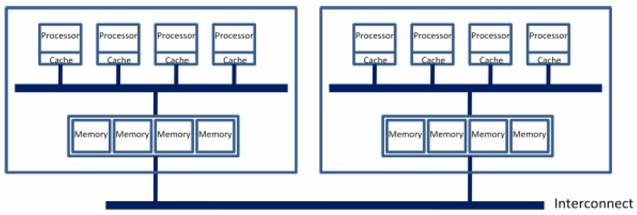
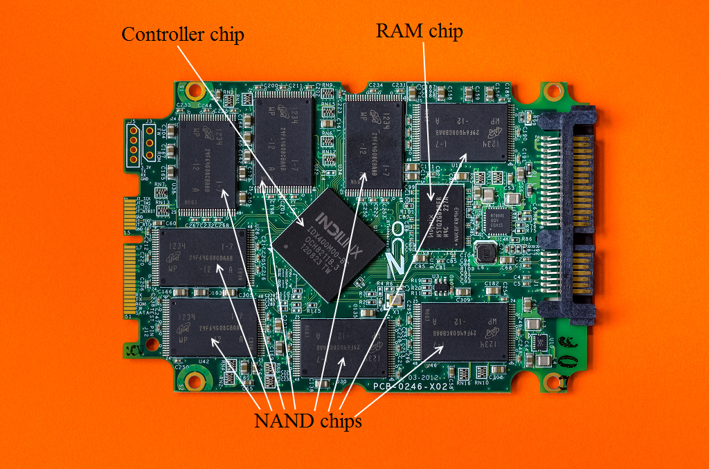(Demo wiki.)

Sys Admin Job Description [From linux.com blog post on 5/20/13 ]

Philosophy of System Administration

Post-install Tasks & Procedures

Logical Volume Management (LVM)

Show Usenix/Sage Policy Docs booklet.

Review disaster recovery web resource.

SLA=service level agreement.

**Discuss Disaster Recovery Project**.

Account and Group Management Commands

Disk Quotas

(Demo wiki.)

Sys Admin Job Description [From linux.com blog post on 5/20/13 ]

Philosophy of System Administration

Post-install Tasks & Procedures

Logical Volume Management (LVM)

Show Usenix/Sage Policy Docs booklet.

Review disaster recovery web resource.

SLA=service level agreement.

Discuss Disaster Recovery Project.

Account and Group Management Commands

Disk Quotas

**Discuss Disaster Recovery Project**.